---

一、Support Vertor Machine 简介

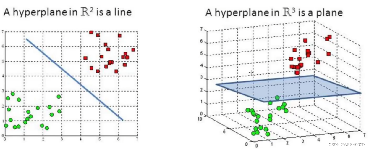
支持向量机（Support Vector Machine, SVM）是一类按监督学习（supervised learning）方式对数据进行二元分类的广义线性分类器（generalized linear classifier），其决策边界是对学习样本求解的最大边距超平面（maximum-margin hyperplane）

它将实例的特征向量映射为空间中的一些点，SVM 的目的就是想要画出一条线，以 “最好地” 区分这两类点，以至如果以后有了新的点，这条线也能做出很好的分类。SVM 适合中小型数据样本、非线性、高维的分类问题。

SVM 最早是由 Vladimir N. Vapnik 和 Alexey Ya. Chervonenkis 在1963年提出，目前的版本（soft margin）是由 Corinna Cortes 和 Vapnik 在1993年提出，并在1995年发表。深度学习（2012）出现之前，SVM 被认为机器学习中近十几年来最成功，表现最好的算法。

二、Support Vertor Machine 详解

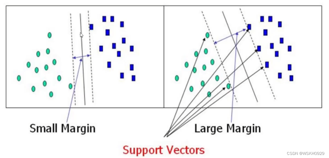
2.1 什么才是好的决策边界

要解决的问题：什么样的决策边界才是最好的呢？

答：决策边界离两个类别的最短距离和越远越好。如下图所示，Large Margin显然是更好的决策边界，因为它具有更强的容错性

2.2 距离与数据定义

2.2.1 点到平面的距离计算

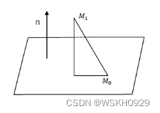
向量法计算点到平面的距离，就是把点和平面放在直角坐标系下进行计算。这样，点 和平面均可用坐标来表示 (如图1所示)。
设平面 $\Pi$ 的方程为:
$$\Pi :Ax+By+Cz+D=0$$
设向量 n ⃗ = ( A , B , C ) vec{n}=(A, B, C) n =(A,B,C) 为 $\Pi$ 的法向量，平面外一点 M 1 M_1 M1​ 坐标为 ( x 1 , y 1 , z 1 ) left(x_1, y_1, z_1right) (x1​,y1​,z1​) ，在平面 上取一点 M 0 M_0 M0​ ，则点 M 1 M_1 M1​ 到平面 $\Pi$ 的距离 $d$ 为:
d = Prj ⁡ n ⃗ M 0 M 1 → = ∥ M 0 M 1 → ∥ cos ⁡ α d=operatorname{Prj}_{vec{n}} overrightarrow{M_0 M_1}=left|overrightarrow{M_0 M_1}right| cos alpha d=Prjn ​M0​M1​ ​=∥ ∥​M0​M1​ ​∥ ∥​cosα
其中 $\alpha$ 为向量 n ⃗ vec{n} n 与向量 M 0 M 1 → overrightarrow{M_0 M_1} M0​M1​ ​ 的夹角，
cos ⁡ α = M 0 M 1 → ⋅ n ⃗ ∥ M 0 M 1 → ∥ ⋅ ∥ n ⃗ ∥ cos alpha=frac{overrightarrow{M_0 M_1} cdot vec{n}}{left|overrightarrow{M_0 M_1}right| cdot|vec{n}|} cosα=∥ ∥​M0​M1​ ​∥ ∥​⋅∥n ∥M0​M1​ ​⋅n ​
故
d = M 0 M 1 → ⋅ n ⃗ ∥ n ⃗ ∥ d=frac{overrightarrow{M_0 M_1} cdot vec{n}}{|vec{n}|} d=∥n ∥M0​M1​ ​⋅n ​

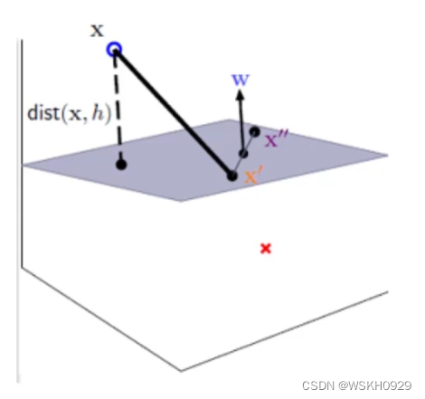
之后统一用下面的方法对距离进行表示：
distance ⁡ ( x , b , w ) = ∣ w T ∥ w ∥ ( x − x ′ ) ∣ = 1 ∥ w ∥ ∣ w T x + b ∣ operatorname{distance}(mathbf{x}, b, mathbf{w})=left|frac{mathbf{w}^T}{|mathbf{w}|}left(mathbf{x}-mathbf{x}^{prime}right)right| { = frac{1}{|mathbf{w}|}}left|mathbf{w}^T mathbf{x}+bright| distance(x,b,w)=∣ ∣​∥w∥wT​(x−x′)∣ ∣​=∥w∥1​∣ ∣​wTx+b∣ ∣​

2.2.2 数据标签定义

数据集 : $(X1,Y1)(X2,Y2)\dots (Xn,Yn)$

$Y$ 为样本的类别: 当 $X$ 为正例时候 $Y=+1$ 当 $X$ 为负例时候 $Y=-1$

决策方程 : y ( x ) = w T Φ ( x ) + b y(x)=w^T Phi(x)+b y(x)=wTΦ(x)+b ( 其中 $\Phi (x)$ 是对数据做了变换，后面继续说 )
⇒ y ( x i ) > 0 ⇔ y i = + 1 y ( x i ) < 0 ⇔ y i = − 1 ⇒ > y i ⋅ y ( x i ) > 0 Rightarrow begin{aligned} &yleft(x_iright)>0 Leftrightarrow y_i=+1 \ &yleft(x_iright)<0 Leftrightarrow y_i=-1 end{aligned} quad Rightarrow>y_i cdot yleft(x_iright)>0 ⇒​y(xi​)>0⇔yi​=+1y(xi​)<0⇔yi​=−1​⇒>yi​⋅y(xi​)>0
可以看出， y i ⋅ y ( x i ) y_i cdot yleft(x_iright) yi​⋅y(xi​)恒为正数，方便后面直接去掉绝对值

2.3 目标函数推导

优化的目标：找到一条线（w和b），使得离该线最近的点能够最远

将点到直线的距离化简得 : y i ⋅ ( w T ⋅ Φ ( x i ) + b ) ∥ w ∥ frac{y_i cdotleft(w^T cdot Phileft(x_iright)+bright)}{|w|} ∥w∥yi​⋅(wT⋅Φ(xi​)+b)​
( 由于 y i ⋅ y ( x i ) > 0 y_i cdot yleft(x_iright)>0 yi​⋅y(xi​)>0 所以将绝对值展开原始依旧成立 )

放缩变换 : 对于决策方程 $(\mathrm{W},\mathrm{b})$ 可以通过放缩使得其结果值 $|\mathrm{Y}|>=1$ ⇒ > y i ⋅ ( w T ⋅ Φ ( x i ) + b ) ≥ 1 Rightarrow>y_i cdotleft(w^T cdot Phileft(x_iright)+bright) geq 1 ⇒>yi​⋅(wT⋅Φ(xi​)+b)≥1 ( 之前我们认为恒大于0，现在严格了些 )

优化目标 : arg ⁡ max ⁡ w , b { 1 ∥ w ∥ min ⁡ i [ y i ⋅ ( w T ⋅ Φ ( x i ) + b ) ] } underset{w, b}{arg max }left{frac{1}{|w|} min _ileft[y_i cdotleft(w^T cdot Phileft(x_iright)+bright)right]right} w,bargmax​{∥w∥1​imin​[yi​⋅(wT⋅Φ(xi​)+b)]}

由于 y i ⋅ ( w T ⋅ Φ ( x i ) + b ) ≥ 1 y_i cdotleft(w^T cdot Phileft(x_iright)+bright) geq 1 yi​⋅(wT⋅Φ(xi​)+b)≥1 ，只需要考虑 arg ⁡ max ⁡ w , b 1 ∥ w ∥ underset{w, b}{arg max } frac{1}{|w|} w,bargmax​∥w∥1​ ( 目标函数搞定！)

2.4 拉格朗日乘子法求解

当前目标 : max ⁡ w , b 1 ∥ w ∥ max _{w, b} frac{1}{|w|} maxw,b​∥w∥1​ ，约束条件 : y i ( w T ⋅ Φ ( x i ) + b ) ≥ 1 y_ileft(w^T cdot Phileft(x_iright)+bright) geq 1 yi​(wT⋅Φ(xi​)+b)≥1

常规套路 : 将求解极大值问题转换成极小值问题 = > m i n w , b 1 2 w 2 =>m i n_{w, b} frac{1}{2} w^2 =>minw,b​21​w2

如何求解 : 应用拉格朗日乘子法求解

带约束的优化问题:
m i n f 0 ( x ) s u b j e c t t o f i ( x ) ≤ 0 , i = 1 , … m h i ( x ) = 0 , i = 1 , … q begin{aligned} min quad &f_0(x) \ subject quad to quad &f_i(x) leq 0, i=1, ldots m \ &h_i(x)=0, i=1, ldots q end{aligned} minsubjectto​f0​(x)fi​(x)≤0,i=1,…mhi​(x)=0,i=1,…q​

原式转换 :

min ⁡ L ( x , λ , v ) = f 0 ( x ) + ∑ i = 1 m λ i f i ( x ) + ∑ i = 1 q v i h i ( x ) min L(x, lambda, v)=f_0(x)+sum_{i=1}^m lambda_i f_i(x)+sum_{i=1}^q v_i h_i(x) minL(x,λ,v)=f0​(x)+i=1∑m​λi​fi​(x)+i=1∑q​vi​hi​(x)

我们的式子:

L ( w , b , α ) = 1 2 ∥ w ∥ 2 − ∑ i = 1 n α i ( y i ( w T ⋅ Φ ( x i ) + b ) − 1 ) L(w, b, alpha)=frac{1}{2}|w|^2-sum_{i=1}^n alpha_ileft(y_ileft(w^T cdot Phileft(x_iright)+bright)-1right) L(w,b,α)=21​∥w∥2−i=1∑n​αi​(yi​(wT⋅Φ(xi​)+b)−1)
 ( 约束条件不要忘 :  y i ( w T ⋅ Φ ( x i ) + b ) ≥ 1 ) text { ( 约束条件不要忘 : } left.y_ileft(w^T cdot Phileft(x_iright)+bright) geq 1right)  ( 约束条件不要忘 : yi​(wT⋅Φ(xi​)+b)≥1)

分别对 $w$ 和 b求偏导，分别得到两个条件 ( 由于对偶性质)

min ⁡ w , b max ⁡ α L ( w , b , α ) → max ⁡ α min ⁡ w , b L ( w , b , α ) min _{w, b} max _alpha L(w, b, alpha) rightarrow max _alpha min _{w, b} L(w, b, alpha) w,bmin​αmax​L(w,b,α)→αmax​w,bmin​L(w,b,α)

对W求偏导:

∂ L ∂ w = 0 ⇒ w = ∑ i = 1 n α i y i Φ ( x n ) frac{partial L}{partial w}=0 Rightarrow w=sum_{i=1}^n alpha_i y_i Phileft(x_nright) ∂w∂L​=0⇒w=i=1∑n​αi​yi​Φ(xn​)

对b求偏导:

∂ L ∂ b = 0 ⇒ ∑ i = 1 n α i y i = 0 quad frac{partial L}{partial b}=0 Rightarrow sum_{i=1}^n alpha_i y_i=0 ∂b∂L​=0⇒i=1∑n​αi​yi​=0

带入原式 :

L ( w , b , α ) = 1 2 ∥ w ∥ 2 − ∑ i = 1 n α i ( y i ( w T Φ ( x i ) + b ) − 1 ) L(w, b, alpha)=frac{1}{2}|w|^2-sum_{i=1}^n alpha_ileft(y_ileft(w^T Phileft(x_iright)+bright)-1right) L(w,b,α)=21​∥w∥2−i=1∑n​αi​(yi​(wTΦ(xi​)+b)−1)

其中:

w = ∑ i = 1 n α i y i Φ ( x n ) 0 = ∑ i = 1 n α i y i 原式 = 1 2 w T w − w T ∑ i = 1 n α i y i Φ ( x i ) − b ∑ i = 1 n α i y i + ∑ i = 1 n α i = ∑ i = 1 n α i − 1 2 ( ∑ i = 1 n α i y i Φ ( x i ) ) T ∑ i = 1 n α i y i Φ ( x i ) = ∑ i = 1 n α i − 1 2 ∑ i = 1 , j = 1 n α i α j y i y j Φ T ( x i ) Φ ( x j ) begin{aligned} w&=sum_{i=1}^n alpha_i y_i Phileft(x_nright) quad 0=sum_{i=1}^n alpha_i y_i \ 原式&=frac{1}{2} w^T w-w^T sum_{i=1}^n alpha_i y_i Phileft(x_iright)-b sum_{i=1}^n alpha_i y_i+sum_{i=1}^n alpha_i \ &=sum_{i=1}^n alpha_i-frac{1}{2}left(sum_{i=1}^n alpha_i y_i Phileft(x_iright)right)^T sum_{i=1}^n alpha_i y_i Phileft(x_iright) \ &=sum_{i=1}^n alpha_i-frac{1}{2} sum_{i=1, j=1}^n alpha_i alpha_j y_i y_j Phi^Tleft(x_iright) Phileft(x_jright) end{aligned} w原式​=i=1∑n​αi​yi​Φ(xn​)0=i=1∑n​αi​yi​=21​wTw−wTi=1∑n​αi​yi​Φ(xi​)−bi=1∑n​αi​yi​+i=1∑n​αi​=i=1∑n​αi​−21​(i=1∑n​αi​yi​Φ(xi​))Ti=1∑n​αi​yi​Φ(xi​)=i=1∑n​αi​−21​i=1,j=1∑n​αi​αj​yi​yj​ΦT(xi​)Φ(xj​)​

继续对 $\alpha$ 求极大值:

max ⁡ α ∑ i = 1 n α i − 1 2 ∑ i = 1 n ∑ j = 1 n α i α j y i y j ( Φ ( x i ) ⋅ Φ ( x j ) ) 条件: ∑ i = 1 n α i y i = 0 α i ≥ 0 max _alpha sum_{i=1}^n alpha_i-frac{1}{2} sum_{i=1}^n sum_{j=1}^n alpha_i alpha_j y_i y_jleft(Phileft(x_iright) cdot Phileft(x_jright)right) \ text{条件:} sum_{i=1}^n alpha_i y_i=0 \ alpha_i geq 0 αmax​i=1∑n​αi​−21​i=1∑n​j=1∑n​αi​αj​yi​yj​(Φ(xi​)⋅Φ(xj​))条件:i=1∑n​αi​yi​=0αi​≥0

极大值转换成求极小值 :

min ⁡ α 1 2 ∑ i = 1 n ∑ j = 1 n α i α j y i y j ( Φ ( x i ) ⋅ Φ ( x j ) ) − ∑ i = 1 n α i 条件: ∑ i = 1 n α i y i = 0 α i ≥ 0 min _alpha frac{1}{2} sum_{i=1}^n sum_{j=1}^n alpha_i alpha_j y_i y_jleft(Phileft(x_iright) cdot Phileft(x_jright)right)-sum_{i=1}^n alpha_i \ text{条件:} sum_{i=1}^n alpha_i y_i=0 \ alpha_i geq 0 αmin​21​i=1∑n​j=1∑n​αi​αj​yi​yj​(Φ(xi​)⋅Φ(xj​))−i=1∑n​αi​条件:i=1∑n​αi​yi​=0αi​≥0

2.5 求解决策方程的例子

下面用一个简单的例子来演示决策方程的求解过程：

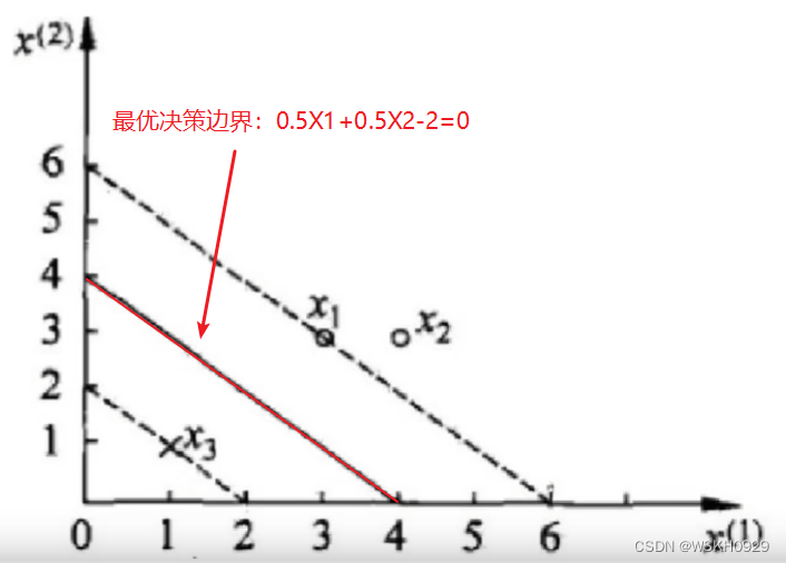
数据：3个点，其中正例X1（3，3），X2（4，3）；负例X3（1，1）

求解 :

1 2 ∑ i = 1 n ∑ j = 1 n α i α j y i y j ( x i ⋅ x j ) − ∑ i = 1 n α i frac{1}{2} sum_{i=1}^n sum_{j=1}^n alpha_i alpha_j y_i y_jleft(x_i cdot x_jright)-sum_{i=1}^n alpha_i 21​i=1∑n​j=1∑n​αi​αj​yi​yj​(xi​⋅xj​)−i=1∑n​αi​

约束条件 :

α 1 + α 2 − α 3 = 0 α i ≥ 0 , i = 1 , 2 , 3 quad alpha_1+alpha_2-alpha_3=0 \ alpha_i geq 0, quad i=1,2,3 α1​+α2​−α3​=0αi​≥0,i=1,2,3

原式:

1 2 ∑ i = 1 n ∑ j = 1 n α i α j y i y j ( x i ⋅ x j ) − ∑ i = 1 n α i frac{1}{2} sum_{i=1}^n sum_{j=1}^n alpha_i alpha_j y_i y_jleft(x_i cdot x_jright)-sum_{i=1}^n alpha_i 21​i=1∑n​j=1∑n​αi​αj​yi​yj​(xi​⋅xj​)−i=1∑n​αi​

将数据代入:

原式 = 1 2 ( 18 α 1 2 + 25 α 2 2 + 2 α 3 2 + 42 α 1 α 2 − 12 α 1 α 3 − 14 α 2 α 3 ) − α 1 − α 2 − α 3 text{原式}=frac{1}{2}left(18 alpha_1^2+25 alpha_2^2+2 alpha_3^2+42 alpha_1 alpha_2-12 alpha_1 alpha_3-14 alpha_2 alpha_3right)-alpha_1-alpha_2-alpha_3 原式=21​(18α12​+25α22​+2α32​+42α1​α2​−12α1​α3​−14α2​α3​)−α1​−α2​−α3​

由于 α 1 + α 2 = α 3 alpha_1+alpha_2=alpha_3 α1​+α2​=α3​ , 化简可得 :

原式 = 4 α 1 2 + 13 2 α 2 2 + 10 α 1 α 2 − 2 α 1 − 2 α 2 text{原式}=4 alpha_1^2+frac{13}{2} alpha_2^2+10 alpha_1 alpha_2-2 alpha_1-2 alpha_2 原式=4α12​+213​α22​+10α1​α2​−2α1​−2α2​

分别对 $\alpha 1$ 和 $\alpha 2$ 求偏导，偏导等于0可得:

α 1 = 1.5 , α 2 = − 1 alpha_1=1.5 , alpha_2=-1 α1​=1.5,α2​=−1

(并不满足约束条件 α i ≥ 0 , i = 1 , 2 , 3 alpha_i geq 0, i=1,2,3 αi​≥0,i=1,2,3 ，所以解应在边界上 )

α 1 = 0 , α 2 = − 2 13 ⇒ 带入原式 = − 0.153 ( 不满足约束 ! ) alpha_1=0 , alpha_2=-frac{2}{13} Rightarrow 带入原式 =-0.153 quad(不满足约束!) α1​=0,α2​=−132​⇒带入原式=−0.153(不满足约束!)

α 1 = 0.25 , α 2 = 0 ⟹ 带入原式 = − 0.25 ( 满足约束 ! ) alpha_1=0.25 , alpha_2=0 quad Longrightarrow quad 带入原式 =-0.25 quad( 满足约束 ! ) α1​=0.25,α2​=0⟹带入原式=−0.25(满足约束!)

综上可得，最小值在 $(0.25,0,0.25)$ 处取得

然后，将 $\alpha$ 结果带入求解: w = ∑ i = 1 n α i y i Φ ( x n ) w=sum_{i=1}^n alpha_i y_i Phileft(x_nright) w=∑i=1n​αi​yi​Φ(xn​)

w = 1 4 ∗ 1 ∗ ( 3 , 3 ) + 1 4 ∗ ( − 1 ) ∗ ( 1 , 1 ) = ( 1 2 , 1 2 ) b = y i − ∑ i = 1 n a i y i ( x i x j ) = 1 − ( 1 4 ∗ 1 ∗ 18 + 1 4 ∗ ( − 1 ) ∗ 6 ) = − 2 begin{aligned} &w=frac{1}{4} * 1 *(3,3)+frac{1}{4} *(-1) *(1,1)=left(frac{1}{2}, frac{1}{2}right) \ &b=y_i-sum_{i=1}^n a_i y_ileft(x_i x_jright)=1-left(frac{1}{4} * 1 * 18+frac{1}{4} *(-1) * 6right)=-2 end{aligned} ​w=41​∗1∗(3,3)+41​∗(−1)∗(1,1)=(21​,21​)b=yi​−i=1∑n​ai​yi​(xi​xj​)=1−(41​∗1∗18+41​∗(−1)∗6)=−2​

最终，求得平面方程为: 0.5 x 1 + 0.5 x 2 − 2 = 0 0.5 x_1+0.5 x_2-2=0 0.5x1​+0.5x2​−2=0

2.6 结合例子深入理解 Support Vertor Machine

结合上面的例子，我们能够更加深入地理解支持向量机。
还记得，在求得的$\alpha$结果中 α 1 = 0.25 , α 2 = 0 , α 3 = 0.25 alpha_1=0.25,alpha_2=0,alpha_3=0.25 α1​=0.25,α2​=0,α3​=0.25

而“巧合”的是，在我们可视化最佳决策边界的图中，我们不难看出，决策边界是由X1和X3所“支撑”起来的，其与X2没有多大关系，所以 α 2 = 0 alpha_2=0 α2​=0是可解释的，因为其不影响到决策边界的确定

这也是为什么这个算法被称为“支持向量机”的原因，因为其求解出的决策边界是由n个向量所支持/支撑起来的。

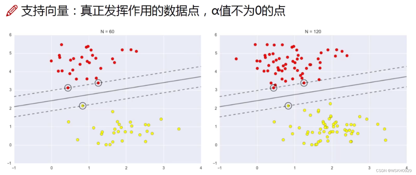
所有$\alpha$值不为0的“边界点”，我们称它们为“支持向量”

2.6 soft-margin 软间隔

有时候数据中有一些噪音点，如果考虑它们，划分出来的决策边界就不太好了

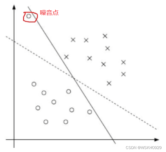
软间隔：之前的方法要求要把两类点完全分得开，这个 要求有点过于严格了，我们来放松一点！

为了解决该问题，引入松弛因子 ξ i xi_i ξi​

y i ( w ⋅ x i + b ) ≥ 1 − ξ i y_ileft(w cdot x_i+bright) geq 1-xi_i yi​(w⋅xi​+b)≥1−ξi​

新的目标函数 :

min ⁡ 1 2 ∥ w ∥ 2 + C ∑ i = 1 n ξ i quad min frac{1}{2}|w|^2+C sum_{i=1}^n xi_i min21​∥w∥2+Ci=1∑n​ξi​

• 当C趋近于很大时：意味着分类严格不能有错误
• 当C趋近于很小时：意味着可以有更大的错误容忍
• C是我们需要指定的一个参数!

修改后的拉格朗日乘子法 :

L ( w , b , ξ , α , μ ) ≡ 1 2 ∥ w ∥ 2 + C ∑ i = 1 n ξ i − ∑ i = 1 n α i ( y i ( w ⋅ x i + b ) − 1 + ξ i ) − ∑ i = 1 n μ i ξ i w = ∑ i = 1 n α i y i ϕ ( x n ) min ⁡ α 1 2 ∑ i = 1 n ∑ j = 1 n α i α j y i y j ( x i ⋅ x j ) − ∑ i = 1 n α i begin{gathered} L(w, b, xi, alpha, mu) equiv frac{1}{2}|w|^2+C sum_{i=1}^n xi_i-sum_{i=1}^n alpha_ileft(y_ileft(w cdot x_i+bright)-1+xi_iright)-sum_{i=1}^n mu_i xi_i \ w=sum_{i=1}^n alpha_i y_i phileft(x_nright) quad quad min _alpha frac{1}{2} sum_{i=1}^n sum_{j=1}^n alpha_i alpha_j y_i y_jleft(x_i cdot x_jright)-sum_{i=1}^n alpha_i end{gathered} L(w,b,ξ,α,μ)≡21​∥w∥2+Ci=1∑n​ξi​−i=1∑n​αi​(yi​(w⋅xi​+b)−1+ξi​)−i=1∑n​μi​ξi​w=i=1∑n​αi​yi​ϕ(xn​)αmin​21​i=1∑n​j=1∑n​αi​αj​yi​yj​(xi​⋅xj​)−i=1∑n​αi​​
约束: 0 = ∑ i = 1 n α i y i 0=sum_{i=1}^n alpha_i y_i quad 0=∑i=1n​αi​yi​ 同样的解法: ∑ i = 1 n α i y i = 0 sum_{i=1}^n alpha_i y_i=0 ∑i=1n​αi​yi​=0
C − α i − μ i = 0 α i ≥ 0 μ i ≥ 0 begin{aligned} &C-alpha_i-mu_i=0 \ &alpha_i geq 0 quad mu_i geq 0 end{aligned} ​C−αi​−μi​=0αi​≥0μi​≥0​
0 ≤ α i ≤ C 0 leq alpha_i leq C 0≤αi​≤C

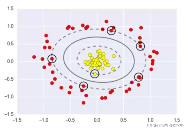
2.7 Kernel Function 核函数

低维空间中线性不可分问题

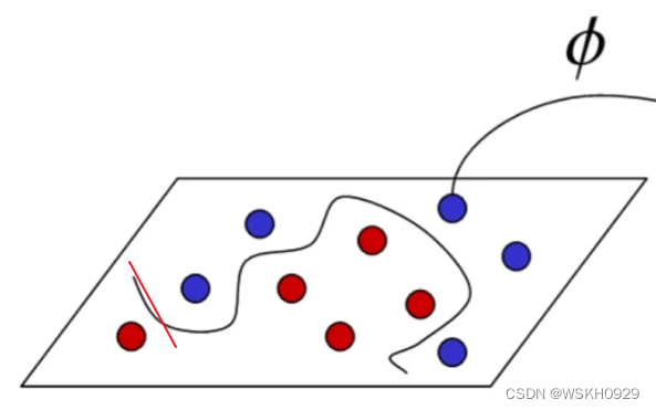
核变换：当低维的时候不可分，那我就给它映射到高维

高斯核函数： K ( X , Y ) = exp ⁡ { − ∥ X − Y ∥ 2 2 σ 2 } K(mathrm{X}, mathrm{Y})=exp left{-frac{|X-Y|^2}{2 sigma^2}right} K(X,Y)=exp{−2σ2∥X−Y∥2​}

三、Support Vertor Machine 代码实战

3.1 支持向量机效果展示

import warnings
import matplotlib.pyplot as plt
import matplotlib
import numpy as np
import os
%matplotlib inline
plt.rcParams['axes.labelsize'] = 14
plt.rcParams['xtick.labelsize'] = 12
plt.rcParams['ytick.labelsize'] = 12
warnings.filterwarnings('ignore')

from sklearn.svm import SVC
from sklearn import datasets

iris = datasets.load_iris()
X = iris['data'][:, (2, 3)]
y = iris['target']
setosa_or_versicolor = (y == 0) | (y == 1)
X = X[setosa_or_versicolor]
y = y[setosa_or_versicolor]
svm_clf = SVC(kernel='linear', C=float('inf'))
svm_clf.fit(X, y)

# 一般的模型
x0 = np.linspace(0, 5.5, 200)
pred_1 = 5*x0-20
pred_2 = x0 - 1.8
pred_3 = 0.1*x0+0.5


def plot_svc_decision_boundary(svm_clf, xmin, xmax, sv=True):
    w = svm_clf.coef_[0]
    b = svm_clf.intercept_[0]
    x0 = np.linspace(xmin, xmax, 200)
    decision_boundary = -w[0]/w[1] * x0 - b/w[1]
    margin = 1/w[1]
    gutter_up = decision_boundary + margin
    gutter_down = decision_boundary - margin
    if sv:
        svs = svm_clf.support_vectors_
        plt.scatter(svs[:, 0], svs[:, 1], s=180, facecolors='#FFAAAA')
    plt.plot(x0, decision_boundary, 'k-', linewidth=2)
    plt.plot(x0, gutter_up, 'k--', linewidth=2)
    plt.plot(x0, gutter_down, 'k--', linewidth=2)


plt.figure(figsize=(14, 4))
plt.subplot(121)
plt.plot(X[:, 0][y == 1], X[:, 1][y == 1], 'bs')
plt.plot(X[:, 0][y == 0], X[:, 1][y == 0], 'ys')
plt.plot(x0, pred_1, 'g--', linewidth=2)
plt.plot(x0, pred_2, 'm-', linewidth=2)
plt.plot(x0, pred_3, 'r-', linewidth=2)
plt.axis([0, 5.5, 0, 2])

plt.subplot(122)
plot_svc_decision_boundary(svm_clf, 0, 5.5)
plt.plot(X[:, 0][y == 1], X[:, 1][y == 1], 'bs')
plt.plot(X[:, 0][y == 0], X[:, 1][y == 0], 'ys')
plt.axis([0, 5.5, 0, 2])

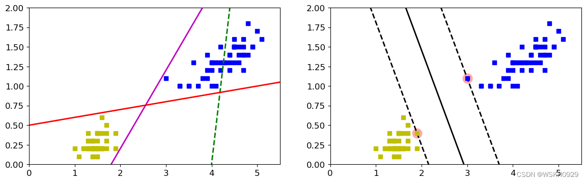
结论：左图为一般线性模型的分类效果，右图为SVM的分类效果，可见SVM的分类效果更好

3.2 软间隔的作用展示

from sklearn.datasets import make_blobs

# 绘图函数
def plot_svc_decision_function(model, ax=None, plot_support=True):
    """Plot the decision function for a 2D SVC"""
    if ax is None:
        ax = plt.gca()
    xlim = ax.get_xlim()
    ylim = ax.get_ylim()

    # create grid to evaluate model
    x = np.linspace(xlim[0], xlim[1], 30)
    y = np.linspace(ylim[0], ylim[1], 30)
    Y, X = np.meshgrid(y, x)
    xy = np.vstack([X.ravel(), Y.ravel()]).T
    P = model.decision_function(xy).reshape(X.shape)

    # plot decision boundary and margins
    ax.contour(X, Y, P, colors='k',
               levels=[-1, 0, 1], alpha=0.5,
               linestyles=['--', '-', '--'])

    # plot support vectors
    if plot_support:
        ax.scatter(model.support_vectors_[:, 0],
                   model.support_vectors_[:, 1],
                   s=300, linewidth=1, facecolors='none')
    ax.set_xlim(xlim)
    ax.set_ylim(ylim)


# 构造数据
X, y = make_blobs(n_samples=100, centers=2,
                  random_state=0, cluster_std=0.8)

fig, ax = plt.subplots(1, 2, figsize=(16, 6))
fig.subplots_adjust(left=0.0625, right=0.95, wspace=0.1)

for axi, C in zip(ax, [10.0, 0.1]):
    model = SVC(kernel='linear', C=C).fit(X, y)
    axi.scatter(model.support_vectors_[:, 0],
            model.support_vectors_[:, 1],
            s=250, lw=1, facecolors='#AFAAAA',alpha=0.5)
    axi.scatter(X[:, 0], X[:, 1], c=y, s=50, cmap='autumn')
    plot_svc_decision_function(model, axi)
    axi.set_title('C = {0:.1f}'.format(C), size=14)

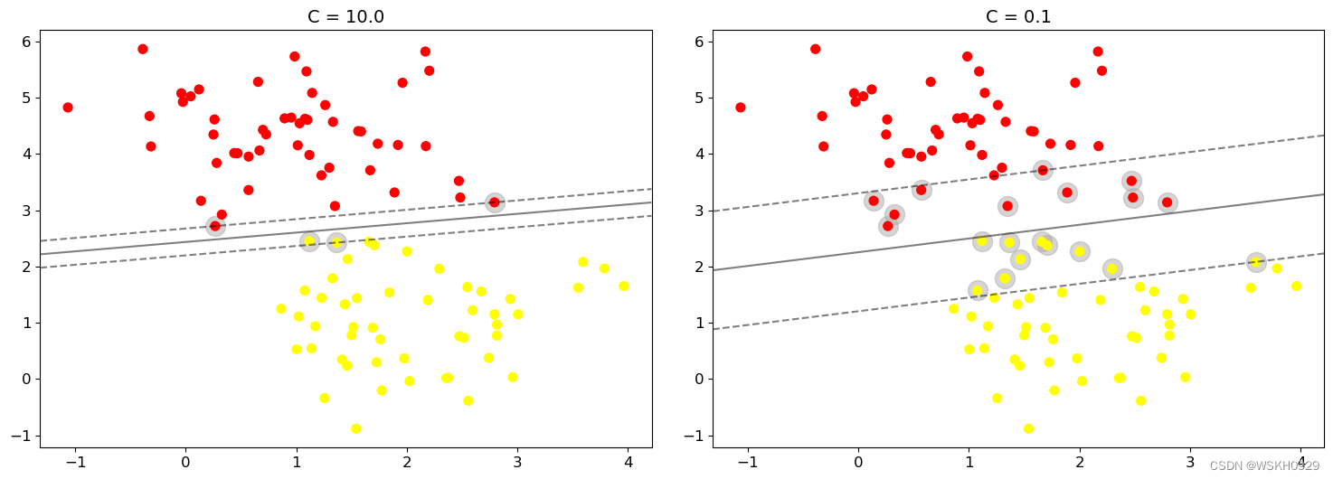
• 当C趋近于无穷大时：意味着分类严格不能有错误
• 当C趋近于很小的时：意味着可以有更大的错误容忍

3.3 非线性 Support Vertor Machine

from sklearn.datasets import make_moons
from sklearn.pipeline import Pipeline
from sklearn.preprocessing import PolynomialFeatures
from sklearn.preprocessing import StandardScaler
from sklearn.svm import LinearSVC

polynomial_svm_clf = Pipeline((("poly_features", PolynomialFeatures(degree=3)),
                              ("scaler", StandardScaler()),
                               ("svm_clf", LinearSVC(C=10, loss="hinge"))
                               ))
polynomial_svm_clf.fit(X, y)


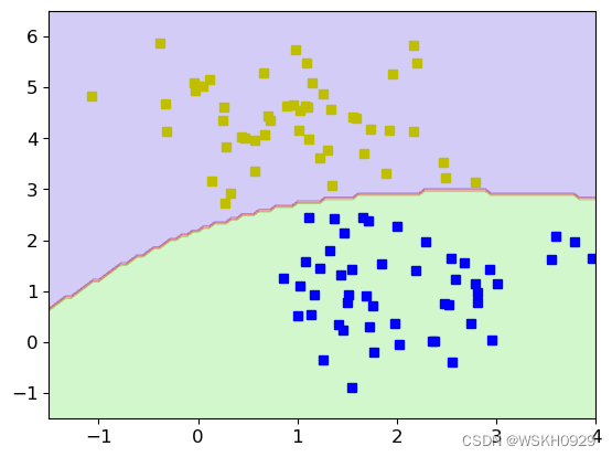
def plot_predictions(clf, axes):
    x0s = np.linspace(axes[0], axes[1], 100)
    x1s = np.linspace(axes[2], axes[3], 100)
    x0, x1 = np.meshgrid(x0s, x1s)
    X = np.c_[x0.ravel(), x1.ravel()]
    y_pred = clf.predict(X).reshape(x0.shape)
    plt.contourf(x0, x1, y_pred, cmap=plt.cm.brg, alpha=0.2)

plt.plot(X[:, 0][y == 1], X[:, 1][y == 1], 'bs')
plt.plot(X[:, 0][y == 0], X[:, 1][y == 0], 'ys')
plot_predictions(polynomial_svm_clf, [-1.5, 4, -1.5, 6.5])

from sklearn.preprocessing import PolynomialFeatures
from sklearn.pipeline import Pipeline
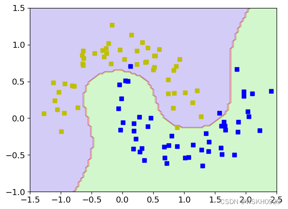
from sklearn.datasets import make_moons

X, y = make_moons(n_samples=100, noise=0.15, random_state=42)


def plot_dataset(X, y, axes):
    plt.plot(X[:, 0][y == 0], X[:, 1][y == 0], "bs")
    plt.plot(X[:, 0][y == 1], X[:, 1][y == 1], "g")
    plt.axis(axes)
    plt.grid(True, which='both')
    plt.xlabel(r"$x_1$", fontsize=20)
    plt.ylabel(r"$x_2$", fontsize=20, rotation=0)
    plot_dataset(X, y, [-1.5, 2.5, -1, 1.5])
    plt.show()


polynomial_svm_clf = Pipeline((("poly_features", PolynomialFeatures(degree=3)),
                               ("scaler", StandardScaler()),
                               ("svm_clf", LinearSVC(C=10, loss="hinge"))))

polynomial_svm_clf.fit(X, y)


def plot_predictions(clf, axes):
    x0s = np.linspace(axes[0], axes[1], 100)
    x1s = np.linspace(axes[2], axes[3], 100)
    x0, x1 = np.meshgrid(x0s, x1s)
    X = np.c_[x0.ravel(), x1.ravel()]
    y_pred = clf.predict(X).reshape(x0.shape)
    plt.contourf(x0, x1, y_pred, cmap=plt.cm.brg, alpha=0.2)


plt.plot(X[:, 0][y == 1], X[:, 1][y == 1], 'bs')
plt.plot(X[:, 0][y == 0], X[:, 1][y == 0], 'ys')
plot_predictions(polynomial_svm_clf, [-1.5, 2.5, -1, 1.5])

3.4 核函数的作用与效果

from sklearn.svm import SVC

poly_kernel_svm_clf = Pipeline([
    ("scaler", StandardScaler()),
    ("svm_clf", SVC(kernel="poly", degree=3, coef0=1, C=5))])
poly_kernel_svm_clf.fit(X, y)

poly100_kernel_svm_clf = Pipeline([
    ("scaler", StandardScaler()),
    ("svm_clf", SVC(kernel="poly", degree=10, coef0=100, C=5))])
poly100_kernel_svm_clf.fit(X, y)

plt.figure(figsize=(16,10))
plt.subplot(221)
plt.title("poly, degree=3, coef0=1")
plt.plot(X[:, 0][y == 1], X[:, 1][y == 1], 'bs')
plt.plot(X[:, 0][y == 0], X[:, 1][y == 0], 'ys')
plot_predictions(poly_kernel_svm_clf, [-1.5, 2.5, -1, 1.5])

plt.subplot(222)
plt.title("poly, degree=10, coef0=100")
plt.plot(X[:, 0][y == 1], X[:, 1][y == 1], 'bs')
plt.plot(X[:, 0][y == 0], X[:, 1][y == 0], 'ys')
plot_predictions(poly100_kernel_svm_clf, [-1.5, 2.5, -1, 1.5])

poly_kernel_svm_clf = Pipeline([
    ("scaler", StandardScaler()),
    ("svm_clf", SVC(kernel="rbf", degree=3, coef0=1, C=5))])
poly_kernel_svm_clf.fit(X, y)

poly100_kernel_svm_clf = Pipeline([
    ("scaler", StandardScaler()),
    ("svm_clf", SVC(kernel="rbf", degree=10, coef0=100, C=5))])
poly100_kernel_svm_clf.fit(X, y)


plt.subplot(223)
plt.title("rbf, degree=3, coef0=1")
plt.plot(X[:, 0][y == 1], X[:, 1][y == 1], 'bs')
plt.plot(X[:, 0][y == 0], X[:, 1][y == 0], 'ys')
plot_predictions(poly_kernel_svm_clf, [-1.5, 2.5, -1, 1.5])

plt.subplot(224)
plt.title("rbf, degree=10, coef0=100")
plt.plot(X[:, 0][y == 1], X[:, 1][y == 1], 'bs')
plt.plot(X[:, 0][y == 0], X[:, 1][y == 0], 'ys')
plot_predictions(poly100_kernel_svm_clf, [-1.5, 2.5, -1, 1.5])

plt.show()

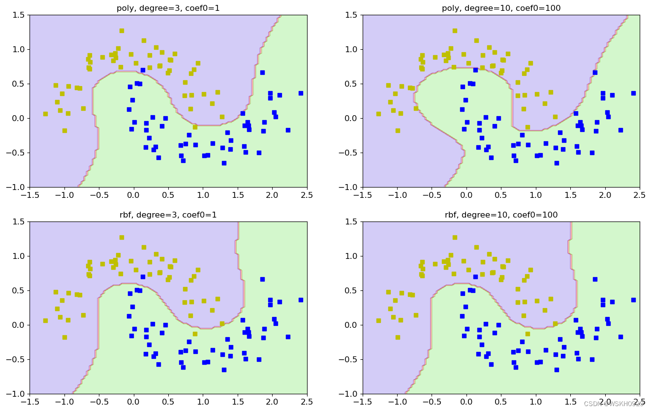
• caef0表示偏置项
• 使用poly核函数的右图的模型过拟合风险更大
• 使用rbf核函数受参数的影响比poly小，并且更不容易过拟合

3.5 Face Recognition 人脸识别案例

作为支持向量机的一个实际例子，让我们来看看面部识别问题。
我们将使用Wild数据集中的Labeled Faces，该数据集包含数千张不同公众人物的整理照片。
数据集的抓取器内置于Scikit Learn中：

3.5.1 获取数据集

from sklearn.datasets import fetch_lfw_people
faces = fetch_lfw_people(min_faces_per_person=60)
print(faces.target_names)
print(faces.images.shape)

输出：

['Ariel Sharon' 'Colin Powell' 'Donald Rumsfeld' 'George W Bush'
 'Gerhard Schroeder' 'Hugo Chavez' 'Junichiro Koizumi' 'Tony Blair']
(1348, 62, 47)

3.5.2 查看人脸图像

fig, ax = plt.subplots(3, 5)
for i, axi in enumerate(ax.flat):
    axi.imshow(faces.images[i], cmap='bone')
    axi.set(xticks=[], yticks=[],
            xlabel=faces.target_names[faces.target[i]])

3.5.3 PCA降维

• 每个图的大小是 [62×47]
• 在这里我们就把每一个像素点当成了一个特征，但是这样特征太多了，用PCA降维一下吧！

from sklearn.svm import SVC
#from sklearn.decomposition import RandomizedPCA
from sklearn.decomposition import PCA
from sklearn.pipeline import make_pipeline

pca = PCA(n_components=150, whiten=True, random_state=42)
svc = SVC(kernel='rbf', class_weight='balanced')
model = make_pipeline(pca, svc)

3.5.4 划分训练集和测试集

from sklearn.model_selection import train_test_split
Xtrain, Xtest, ytrain, ytest = train_test_split(faces.data, faces.target,
                                                random_state=40)

3.5.5 网格搜索训练

使用grid search cross-validation来选择较好的参数

from sklearn.model_selection import GridSearchCV
param_grid = {'svc__C': [1, 5, 10],
              'svc__gamma': [0.0001, 0.0005, 0.001]}
grid = GridSearchCV(model, param_grid)

%time grid.fit(Xtrain, ytrain)
print(grid.best_params_)

输出：

CPU times: total: 1min 18s
Wall time: 13.3 s
{'svc__C': 5, 'svc__gamma': 0.001}

3.5.6 为模型设置最佳参数并预测图片类别

model = grid.best_estimator_
yfit = model.predict(Xtest)

3.5.7 可视化分类结果

fig, ax = plt.subplots(4, 6)
for i, axi in enumerate(ax.flat):
    axi.imshow(Xtest[i].reshape(62, 47), cmap='bone')
    axi.set(xticks=[], yticks=[])
    axi.set_ylabel(faces.target_names[yfit[i]].split()[-1],
                   color='black' if yfit[i] == ytest[i] else 'red')
fig.suptitle('Predicted Names; Incorrect Labels in Red', size=14);

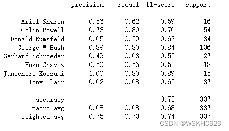
3.5.8 输出每个类别预测的准确率、召回率等信息

• 精度(precision) = 正确预测的个数(TP)/被预测正确的个数(TP+FP)
• 召回率(recall)=正确预测的个数(TP)/预测个数(TP+FN)
• F1 = 2精度召回率/(精度+召回率)

from sklearn.metrics import classification_report
print(classification_report(ytest, yfit,
                            target_names=faces.target_names))

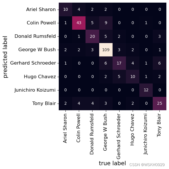
3.5.9 绘制混淆矩阵

from sklearn.metrics import confusion_matrix
import seaborn as sns
mat = confusion_matrix(ytest, yfit)
sns.heatmap(mat.T, square=True, annot=True, fmt='d', cbar=False,
            xticklabels=faces.target_names,
            yticklabels=faces.target_names)
plt.xlabel('true label')
plt.ylabel('predicted label');