Soft Actor Critic算法论文公式详解

SAC强化学习算法是伯克利大学团队2018年在ICML(International Conference on Machine Learning)上发表的论文，本篇博客来总结一下论文里的公式及其涵义。

论文地址：Soft Actor-Critic: Off-Policy Maximum Entropy Deep Reinforcement Learning with a Stochastic Actor

1. 符号说明

马尔科夫决策过程：$$(\mathcal{S},\mathcal{A},p,r)$$其中，$\mathcal{S}$为状态空间；$\mathcal{A}$为动作空间；未知的状态转移概率$p:\mathcal{S}\times \mathcal{S}\times \mathcal{A}\to [0,\infty )$表示给定当前状态 s t ∈ S s_tinmathcal{S} st​∈S和动作 a t ∈ A a_tin mathcal{A} at​∈A时下一个状态 s t + 1 ∈ S s_{t+1}in mathcal{S} st+1​∈S的概率密度；环境在每次状态转移时获得一个有界的立即回报 r : S × A → [ r min ⁡ , r max ⁡ ] r:mathcal{S}timesmathcal{A}to[r_{min}, r_{max}] r:S×A→[rmin​,rmax​]； ρ π ( s t ) rho_{pi}(s_t) ρπ​(st​)和 ρ π ( s t , a t ) rho_{pi}(s_t,a_t) ρπ​(st​,at​)分别表示由策略 π ( a t ∣ s t ) pi(a_t|s_t) π(at​∣st​)产生的轨迹的边缘状态、状态-动作分布(边缘即当前时刻的意思)。

1. 累计平均回报

SAC算法设定了一个最大熵目标 r ( s t , a t ) + α H ( π ( ⋅ ∣ s t ) ) r(s_t,a_t)+alphamathcal{H}(pi(·|s_t)) r(st​,at​)+αH(π(⋅∣st​))，它通过最大化累计最大熵目标的期望值$J(\pi )$（累计平均回报）来使策略$\pi$随机化，如公式(1)：
J ( π ) = ∑ t = 0 T E ( s t , a t ) ∼ ρ π [ r ( s t , a t ) + α H ( π ( ⋅ ∣ s t ) ) ] J(pi)=sum_{t=0}^{T}mathbb{E}_{(s_t,a_t)simrho_pi}[r(s_t,a_t)+alphamathcal{H}(pi(·|s_t))] J(π)=t=0∑T​E(st​,at​)∼ρπ​​[r(st​,at​)+αH(π(⋅∣st​))]其中， r ( s t , a t ) r(s_t,a_t) r(st​,at​)表示普通的立即回报项； H ( π ( ⋅ ∣ s t ) ) mathcal{H}(pi(·|s_t)) H(π(⋅∣st​))表示熵回报项；$\alpha$是温度参数(权重)，它决定了熵项对立即回报的相对重要性，从而控制了最优策略的随机性，在下文中凡是涉及到熵项的都应带上权重$\alpha$，只是有时会略写。

1.1. 熵探索策略

熵回报项 H ( π ( ⋅ ∣ s t ) ) mathcal{H}(pi(·|s_t)) H(π(⋅∣st​))是如何产生随机策略的？我们来看到信息熵的数学公式： H ( X ) = E [ − log ⁡ P ( X ) ] = − E x i log ⁡ P ( x i ) mathcal{H}(X)=mathbb{E}[-log P(X)]=-mathbb{E}_{x_i}log P(x_i) H(X)=E[−logP(X)]=−Exi​​logP(xi​)其中， x i x_i xi​是随机变量； P ( x i ) P(x_i) P(xi​)是随机变量出现的概率。需要注意，由于概率值 P ( x i ) ∈ [ 0 , 1 ] P(x_i)in [0,1] P(xi​)∈[0,1]，因此 log ⁡ P ( x i ) ⩽ 0 log P(x_i)leqslant 0 logP(xi​)⩽0，即$\mathcal{H}(X)⩾0$。

当我们使用随机策略而不是确定性策略时，策略 π ( s t , a t ) pi(s_t,a_t) π(st​,at​)就代表在状态 s t s_t st​时 a t a_t at​被选择的概率。此时可得推导式(1)： H ( π ( ⋅ ∣ s t ) ) = − E a t ∼ π log ⁡ π ( a t ∣ s t ) = − log ⁡ π ( ⋅ ∣ s t ) mathcal{H}(pi(cdot|s_{t}))=-mathbb{E}_{a_tsim pi}log pi(a_t|s_t)=-log pi(·|s_t) H(π(⋅∣st​))=−Eat​∼π​logπ(at​∣st​)=−logπ(⋅∣st​)

可以看到，策略$\pi$产生的动作越确定，即某些动作被选择的概率远大于其他大部分动作，那么其他大部分动作被选择的概率就相对较小，熵期望值就会越大；反之，若策略$\pi$产生的动作越不确定，即各个动作被选择的概率较为平均，熵值就越趋向于0。

可能上面的话不是很直观，下面我们举个例子。假设现在有5个动作可供选择，不同策略$\pi$产生动作的概率分别有以下两种情况：

pi_1 = [0.2, 0.2, 0.2, 0.2, 0.2];
pi_2 = [0.1, 0.1, 0.6, 0.1, 0.1];

下图分别是两种策略产生动作概率的示意图，柱子上面的数字就是该动作当前概率下的熵值，所有动作熵值求期望之后就得到了该策略的熵值。

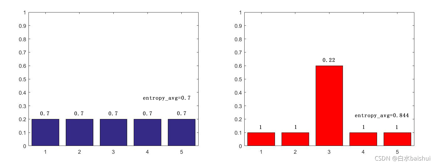
可以看出，左图的 H ( π 1 ( ⋅ ∣ s t ) ) = 0.7 mathcal{H}(pi_1(cdot|s_{t}))=0.7 H(π1​(⋅∣st​))=0.7，要小于右图的 H ( π 2 ( ⋅ ∣ s t ) ) = 0.844 mathcal{H}(pi_2(cdot|s_{t}))=0.844 H(π2​(⋅∣st​))=0.844。

熵探索的特性有利于加快策略的收敛速度(朝熵值最大化的方向收敛)，同时由于动作的选择是概率性的，因此策略可以进行更广泛的探索，当有多个较优动作时(即概率值较高且接近)，可以获取多个较优动作而不是选择最优的一个。

1.2. 附录A：无限马尔科夫决策过程

公式(1) 所描述的优化目标是一次交互的最大熵目标，若要将优化目标扩展为无限马尔科夫决策过程，且允许交互轨迹不完整，则要引入折扣因子$\gamma$，这时优化目标$J(\pi )$定义为公式(14)： J ( π ) = ∑ t = 0 ∞ E ( s t , a t ) ∼ ρ π [ ∑ l = t ∞ γ l − t E s l ∼ p , a l ∼ π [ r ( s t , a t ) + α H ( π ( ⋅ ∣ s t ) ) ] ] J(pi)=sum_{t=0}^{infty}mathbb{E}_{(s_t,a_t)simrho_pi}biggl[sum_{l=t}^{infty}gamma^{l-t}mathbb{E}_{s_lsim p,a_lsim pi}[r(s_t,a_t)+alphamathcal{H}(pi(·|s_t))]biggr] J(π)=t=0∑∞​E(st​,at​)∼ρπ​​[l=t∑∞​γl−tEsl​∼p,al​∼π​[r(st​,at​)+αH(π(⋅∣st​))]]

这样的定义是将未来的回报全部折现到$l=t$时刻，从这个角度理解，公式(1) 与公式(14) 就可以进行如下对比：
J ( π ) T = ∑ t = 0 T E ( s t , a t ) ∼ ρ π [ G t c u r ] J(pi)^T=sum_{t=0}^{T}mathbb{E}_{(s_t,a_t)simrho_pi}[G_t^{cur}] J(π)T=t=0∑T​E(st​,at​)∼ρπ​​[Gtcur​] J ( π ) ∞ = ∑ t = 0 ∞ E ( s t , a t ) ∼ ρ π [ G t d i s ] J(pi)^infty=sum_{t=0}^{infty}mathbb{E}_{(s_t,a_t)simrho_pi}[G_t^{dis}] J(π)∞=t=0∑∞​E(st​,at​)∼ρπ​​[Gtdis​] G t c u r G_t^{cur} Gtcur​只包括了状态 s t s_t st​时的现值回报， G t d i s G_t^{dis} Gtdis​包括了当前状态 s t s_t st​时的现值回报以及未来$\infty -l$个状态的折现回报。虽然我这里写的是$\infty -l$，但实际上，由于 γ l − t gamma^{l-t} γl−t在不断减小，$\infty$一定是有一个大于$l$的终止值的。

2. Soft 策略迭代

最大熵策略的策略迭代过程称为Soft策略迭代，它分为两个步骤：(1)Soft 策略评估；(2)Soft 策略改进。

在Soft策略迭代中，对于固定的策略$\pi$，任何函数$Q:\mathcal{S}\times \mathcal{A}\to \mathbb{R}$开始，应用贝尔曼算子 T π mathcal{T}^pi Tπ可得Soft Q值，表示为公式(2)：
T π Q ( s t , a t ) ≜ r ( a t , s t ) + γ E s t + 1 ∼ p [ V ( s t + 1 ) ] mathcal{T}^{pi}Q(s_t,a_t)triangleq r(a_t,s_t)+gammamathbb{E}_{s_{t+1}sim p}[V(s_{t+1})] TπQ(st​,at​)≜r(at​,st​)+γEst+1​∼p​[V(st+1​)]其中，状态-值函数 V ( s t + 1 ) V(s_{t+1}) V(st+1​)由公式(3) 表示：
V ( s t ) = E a t ∼ π [ Q ( s t , a t ) − log ⁡ ( π ( a t ∣ s t ) ) ] V(s_t)=mathbb{E}_{a_tsimpi}[Q(s_t,a_t)-log(pi(a_t|s_t))] V(st​)=Eat​∼π​[Q(st​,at​)−log(π(at​∣st​))]这里的状态-值函数称为Soft V函数，通过重复应用贝尔曼算子 T π mathcal{T}^pi Tπ，得到任何策略$\pi$的Soft V函数。

贝尔曼算子 T π mathcal{T}^pi Tπ是一种操作符，它表示对当前的价值函数集 $V$ 利用贝尔曼方程进行更新。

2.1. Soft V函数的推导过程

由强化学习的定义可知，$V$函数是指状态值函数，表示状态 s t s_t st​时的价值；$Q$函数是指状态-动作-值函数，表示在状态 s t s_t st​时执行的动作 a t a_t at​的价值，它们之间有如下关系： V ( s t ) = E a t ∼ π [ Q ( s t , a t ) ] V(s_t)=mathbb{E}_{a_tsimpi}[Q(s_t,a_t)] V(st​)=Eat​∼π​[Q(st​,at​)]也即，$V$函数等于$Q$函数对动作求期望。但这个公式中的$Q$函数是不含熵项的，而SAC所采用的最大熵回报中含有熵项，因此需要将熵值加入到$Q$函数的值中，这个$Q$函数才是soft $Q$函数，才能得出soft $V$函数的值，再结合推导式(1)，最终表达为公式(3)：

V ( s t ) = E a t ∼ π [ Q ( s t , a t ) + H ( π ( ⋅ ∣ s t ) ) ] = E a t ∼ π [ Q ( s t , a t ) − log ⁡ ( π ( a t ∣ s t ) ) ] begin{aligned} V(s_t) & = mathbb{E}_{a_tsimpi}[Q(s_t,a_t)+mathcal{H}(pi(·|s_t))] \ & = mathbb{E}_{a_tsimpi}[Q(s_t,a_t)-log(pi(a_t|s_t))] \ end{aligned} V(st​)​=Eat​∼π​[Q(st​,at​)+H(π(⋅∣st​))]=Eat​∼π​[Q(st​,at​)−log(π(at​∣st​))]​

2.2. 引理1：Soft 策略评估

由于在$Q$函数的映射 Q 0 : S × A → R Q^0:mathcal{S}timesmathcal{A}tomathbb{R} Q0:S×A→R中，动作空间$|\mathcal{A}|<\infty$，即动作空间有限，因此由**公式(2)**所定义的Soft Q值更新公式 Q k + 1 = T π Q k Q^{k+1}=mathcal{T}^{pi}Q^k Qk+1=TπQk在固定策略$\pi$下，当$k\to \infty$时一定是收敛的。

2.2.2. 引理1：Soft 策略评估的收敛性证明

首先，将当前策略$\pi$下的立即回报记为： r π ( s t , a t ) ≜ r ( s t , a t ) + E s t + 1 ∼ p [ α H ( π ( ⋅ ∣ s t ) ) ] r_pi(s_t,a_t)triangleq r(s_t,a_t)+mathbb{E}_{s_{t+1}sim p}[alphamathcal{H}(pi(·|s_t))] rπ​(st​,at​)≜r(st​,at​)+Est+1​∼p​[αH(π(⋅∣st​))]注意，原文的这个公式没有写熵的权重$\alpha$，是作者省略了，而不是它不存在。另外，由于策略$\pi$确定，因此 a t = π ( s t ) a_t=pi(s_t) at​=π(st​)确定，所以无需再强调策略的期望值 E a t ∼ π mathbb{E}_{a_tsim pi} Eat​∼π​。

那么此时Soft Q函数的更新公式就表示为公式(15)： Q ( s t , a t ) ← r π ( s t , a t ) + γ E s t + 1 ∼ p , a t + 1 ∼ π [ Q ( s t + 1 , a t + 1 ) ] Q(s_t,a_t)leftarrow r_pi(s_t,a_t)+gammamathbb{E}_{s_{t+1}sim p,a_{t+1}sim pi}[Q(s_{t+1},a_{t+1})] Q(st​,at​)←rπ​(st​,at​)+γEst+1​∼p,at+1​∼π​[Q(st+1​,at+1​)]在公式(15) 中，若满足动作空间$|\mathcal{A}|<\infty$，则 r π ( s t , a t ) r_pi(s_t,a_t) rπ​(st​,at​)是有限的，且当$k\to \infty$时，$\gamma$值逐渐减小，保证了 Q ( s t , a t ) Q(s_t,a_t) Q(st​,at​)是有界的。

2.2.3. 引理1：Soft 策略评估的收敛性证明的推导过程

尽管原文写了收敛性的最终导出，但是省略了一些中间步骤，在这里补上。
首先由公式(2) 和公式(3) 和推导式(1) 可得推导式(2)： { T π Q ( s t , a t ) ≜ r ( a t , s t ) + γ E s t + 1 ∼ p [ V ( s t + 1 ) ] V ( s t ) = E a t ∼ π [ Q ( s t , a t ) − log ⁡ ( π ( a t ∣ s t ) ) ] H ( π ( ⋅ ∣ s t ) ) = − E a t ∼ π log ⁡ π ( a t ∣ s t ) ⇒ begin{cases} mathcal{T}^{pi}Q(s_t,a_t)triangleq r(a_t,s_t)+gammamathbb{E}_{s_{t+1}sim p}[V(s_{t+1})] \ V(s_t)=mathbb{E}_{a_tsimpi}[Q(s_t,a_t)-log(pi(a_t|s_t))] \ mathcal{H}(pi(cdot|s_{t}))=-mathbb{E}_{a_tsim pi}log pi(a_t|s_t) end{cases}Rightarrow ⎩⎪⎨⎪⎧​TπQ(st​,at​)≜r(at​,st​)+γEst+1​∼p​[V(st+1​)]V(st​)=Eat​∼π​[Q(st​,at​)−log(π(at​∣st​))]H(π(⋅∣st​))=−Eat​∼π​logπ(at​∣st​)​⇒

T π Q ( s t , a t ) ≜ r ( a t , s t ) + γ E s t + 1 ∼ p [ E a t ∼ π Q ( s t + 1 , a t + 1 ) + H ( π ( ⋅ ∣ s t ) ) ] = π ( s t ) r ( a t , s t ) + γ E s t + 1 ∼ p [ H ( π ( ⋅ ∣ s t ) ) ] + γ E s t + 1 ∼ p , a t + 1 ∼ π [ Q ( s t + 1 , a t + 1 ) ] = γ 0 = 1 r ( a t , s t ) + E s t + 1 ∼ p [ H ( π ( ⋅ ∣ s t ) ) ] + γ E s t + 1 ∼ p , a t + 1 ∼ π [ Q ( s t + 1 , a t + 1 ) ] = r π ( s t , a t ) + γ E s t + 1 ∼ p , a t + 1 ∼ π [ Q ( s t + 1 , a t + 1 ) ] Q ( s t , a t ) ← r π ( s t , a t ) + γ E s t + 1 ∼ p , a t + 1 ∼ π [ Q ( s t + 1 , a t + 1 ) ] begin{aligned} mathcal{T}^{pi}Q(s_t,a_t) & triangleq r(a_t,s_t)+gammamathbb{E}_{s_{t+1}sim p}[mathbb{E}_{a_tsimpi}Q(s_{t+1},a_{t+1})+mathcal{H}(pi(·|s_t))] \ & overset{pi(s_t)}{=} r(a_t,s_t)+gammamathbb{E}_{s_{t+1}sim p}[mathcal{H}(pi(·|s_t))]+gammamathbb{E}_{s_{t+1}sim p,a_{t+1}simpi}[Q(s_{t+1},a_{t+1})] \ & overset{gamma^0=1}{=} r(a_t,s_t)+mathbb{E}_{s_{t+1}sim p}[mathcal{H}(pi(·|s_t))]+gammamathbb{E}_{s_{t+1}sim p,a_{t+1}simpi}[Q(s_{t+1},a_{t+1})] \ & = r_pi(s_t,a_t)+gammamathbb{E}_{s_{t+1}sim p,a_{t+1}simpi}[Q(s_{t+1},a_{t+1})] \ Q(s_t,a_t)& leftarrow r_pi(s_t,a_t)+gammamathbb{E}_{s_{t+1}sim p,a_{t+1}sim pi}[Q(s_{t+1},a_{t+1})] \ end{aligned} TπQ(st​,at​)Q(st​,at​)​≜r(at​,st​)+γEst+1​∼p​[Eat​∼π​Q(st+1​,at+1​)+H(π(⋅∣st​))]=π(st​)r(at​,st​)+γEst+1​∼p​[H(π(⋅∣st​))]+γEst+1​∼p,at+1​∼π​[Q(st+1​,at+1​)]=γ0=1r(at​,st​)+Est+1​∼p​[H(π(⋅∣st​))]+γEst+1​∼p,at+1​∼π​[Q(st+1​,at+1​)]=rπ​(st​,at​)+γEst+1​∼p,at+1​∼π​[Q(st+1​,at+1​)]←rπ​(st​,at​)+γEst+1​∼p,at+1​∼π​[Q(st+1​,at+1​)]​

再稍微解释一下，第一步，由于策略$\pi$是确定的 s t s_t st​状态下的策略，因此带入的时候不需要把 H ( π ( ⋅ ∣ s t ) ) mathcal{H}(pi(·|s_t)) H(π(⋅∣st​))写成 H ( π ( ⋅ ∣ s t + 1 ) ) mathcal{H}(pi(·|s_{t+1})) H(π(⋅∣st+1​))

第一步到第二步是由于$t$时刻的策略$\pi$是确定的，因此在状态 s t s_t st​时，动作 a t = π ( s t ) a_t=pi(s_t) at​=π(st​)是确定的，无需再估算动作的期望值；

第二步到第三步是由于 E s t + 1 ∼ p [ H ( π ( ⋅ ∣ s t ) ) ] mathbb{E}_{s_{t+1}sim p}[mathcal{H}(pi(·|s_t))] Est+1​∼p​[H(π(⋅∣st​))]是立即回报值的一部分，不需要进行折扣， γ ≜ γ 0 = 1 gammatriangleq gamma^0=1 γ≜γ0=1；

第三部到第四部由2.1.2.中提到的公式 r π ( s t , a t ) ≜ r ( s t , a t ) + E s t + 1 ∼ p [ α H ( π ( ⋅ ∣ s t ) ) ] r_pi(s_t,a_t)triangleq r(s_t,a_t)+mathbb{E}_{s_{t+1}sim p}[alphamathcal{H}(pi(·|s_t))] rπ​(st​,at​)≜r(st​,at​)+Est+1​∼p​[αH(π(⋅∣st​))]得到。

2.3. Soft 策略改进

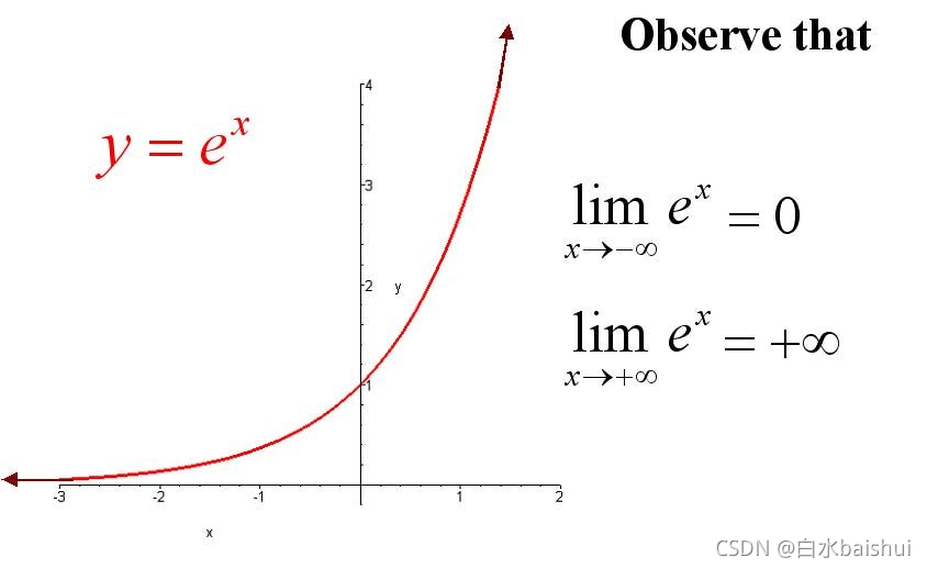
Soft 策略$\pi$ 是通过Soft Q值的相对大小来给动作赋予被选择的概率的，因此在Soft 策略改进中，首先需要将预测Soft Q值转化到指数函数上，这样保证了概率的非负性。
exp ⁡ ( Q π ( s t , ⋅ ) ) exp(Q^pi(s_t,·)) exp(Qπ(st​,⋅))

下一步，为了确保各个Soft Q值转化后的概率之和等于1。需要将转换后的结果进行归一化处理。方法就是将转化后的结果除以所有转化后结果之和，可以理解为转化后结果占总数的百分比。这样就得到近似的概率。 exp ⁡ ( Q π ( s t , ⋅ ) ) Z π ( s t ) frac{exp(Q^{pi}(s_t,·))}{Z^{pi}(s_t)} Zπ(st​)exp(Qπ(st​,⋅))​实际上，这个策略$\pi$产生动作概率的过程就是一个SoftMax的过程，最终结果就是输出了当前策略$\pi$时每个动作被选择概率的分布情况。

到这里，由旧策略 π o l d pi_{old} πold​向新策略 π n e w pi_{new} πnew​更新的过程就可以表示为公式(4)：

π n e w = arg min ⁡ π ′ ∈ ∏ D K L ( π ′ ( ⋅ ∣ s t ) ∥ exp ⁡ ( Q π o l d ( s t , ⋅ ) ) Z π o l d ( s t ) ) pi_{new}=argmin_{pi'inprod}D_{KL}Bigl(pi'(·|s_t)Vertfrac{exp(Q^{pi_{old}}(s_t,·))}{Z^{pi_{old}}(s_t)}Bigr) πnew​=π′∈∏argmin​DKL​(π′(⋅∣st​)∥Zπold​(st​)exp(Qπold​(st​,⋅))​)这个更新公式使用了KL散度来做分布投影，简单来说，KL散度的作用就是衡量两个分布之间的差异。通过在策略空间$\prod$(所有动作概率值的组合空间)中，寻找与 exp ⁡ ( Q π ( s t , ⋅ ) ) Z π ( s t ) frac{exp(Q^{pi}(s_t,·))}{Z^{pi}(s_t)} Zπ(st​)exp(Qπ(st​,⋅))​最相似的分布 π ′ pi' π′来作为新的策略 π n e w = π ′ ∈ ∏ pi_{new}=pi'inprod πnew​=π′∈∏。

注意这里的 exp ⁡ ( Q π ( s t , ⋅ ) ) Z π ( s t ) frac{exp(Q^{pi}(s_t,·))}{Z^{pi}(s_t)} Zπ(st​)exp(Qπ(st​,⋅))​虽然产生自 π o l d pi_{old} πold​，但由于策略的随机性， exp ⁡ ( Q π ( s t , ⋅ ) ) Z π ( s t ) frac{exp(Q^{pi}(s_t,·))}{Z^{pi}(s_t)} Zπ(st​)exp(Qπ(st​,⋅))​并不完全等于 π o l d pi_{old} πold​。

2.3.1. 引理2：Soft 策略改进

设 π o l d ∈ ∏ pi_{old}inprod πold​∈∏以及 π n e w pi_{new} πnew​是由公式(4) 生成当前状态 s t s_t st​下的最优策略。那么当满足 ( s t , a t ) ∈ S × A (s_t,a_t)in mathcal{S}timesmathcal{A} (st​,at​)∈S×A且$|\mathcal{A}|<\infty$时一定会有 Q π n e w ( s t , a t ) ⩾ Q π n e w ( s t , a t ) Q^{pi_{new}}(s_t,a_t)geqslant Q^{pi_{new}}(s_t,a_t) Qπnew​(st​,at​)⩾Qπnew​(st​,at​)

2.3.2. 引理2：Soft 策略改进证明

首先，我们定义 Q π o l d Q^{pi_{old}} Qπold​和 V π o l d V^{pi_{old}} Vπold​是在策略 π o l d pi_{old} πold​下产生的Soft Q值和Soft V值，那么有公式(4) 可得公式(16)：
π n e w = arg min ⁡ π ′ ∈ ∏ D K L ( π ′ ( ⋅ ∣ s t ) ∥ exp ⁡ ( Q π o l d ( s t , ⋅ ) ) Z π o l d ( s t ) ) = arg min ⁡ π ′ ∈ ∏ D K L ( π ′ ( ⋅ ∣ s t ) ∥ exp ⁡ ( Q π o l d ( s t , ⋅ ) − log ⁡ Z π o l d ( s t ) ) ) = arg min ⁡ π ′ ∈ ∏ J π o l d ( π ′ ( ⋅ ∣ s t ) ) begin{aligned} pi_{new} &=argmin_{pi'inprod}D_{KL}Bigl(pi'(·|s_t)Vertfrac{exp(Q^{pi_{old}}(s_t,·))}{Z^{pi_{old}}(s_t)}Bigr) \ & = argmin_{pi'inprod}D_{KL}Bigl(pi'(·|s_t)Vertexp(Q^{pi_{old}}(s_t,·)-log Z^{pi_{old}}(s_t))Bigr) \ & = argmin_{pi'inprod} J_{pi_{old}}(pi'(·|s_t)) \ end{aligned} πnew​​=π′∈∏argmin​DKL​(π′(⋅∣st​)∥Zπold​(st​)exp(Qπold​(st​,⋅))​)=π′∈∏argmin​DKL​(π′(⋅∣st​)∥exp(Qπold​(st​,⋅)−logZπold​(st​)))=π′∈∏argmin​Jπold​​(π′(⋅∣st​))​其中， J π o l d ( π ′ ( ⋅ ∣ s t ) ) J_{pi_{old}}(pi'(·|s_t)) Jπold​​(π′(⋅∣st​))是指 π o l d pi_{old} πold​在当前状态 s t s_t st​时所产生的动作概率分布与 π ′ ( ⋅ ∣ s t ) pi'(·|s_t) π′(⋅∣st​)的KL散度，也就是它们之间的差异大小。

并不显而易见的是，由公式(16) 一定导出这样的情况： J π o l d ( π n e w ( ⋅ ∣ s t ) ) ⩽ J π o l d ( π o l d ( ⋅ ∣ s t ) ) J_{pi_{old}}(pi_{new}(·|s_t))leqslant J_{pi_{old}}(pi_{old}(·|s_t)) Jπold​​(πnew​(⋅∣st​))⩽Jπold​​(πold​(⋅∣st​))初一看这个公式好像有点反直觉， π o l d pi_{old} πold​与 π n e w ( ⋅ ∣ s t ) pi_{new}(·|s_t) πnew​(⋅∣st​)的KL散度怎么会小于 π o l d pi_{old} πold​与 π o l d ( ⋅ ∣ s t ) pi_{old}(·|s_t) πold​(⋅∣st​)的KL散度呢？明明 π o l d pi_{old} πold​与 π o l d pi_{old} πold​的分布是一样的，KL散度不应该对于0吗？但实际上，策略 π o l d pi_{old} πold​产生的是随机策略，因此它作为一个固定策略不一定能很好的表示当前状态 s t s_t st​时它自身产生的动作概率分布，正相反，由于 π n e w ( ⋅ ∣ s t ) pi_{new}(·|s_t) πnew​(⋅∣st​)是当前状态 s t s_t st​时动作概率分布的近似分布。因此在当前的状态 s t s_t st​时，有 J π o l d ( π n e w ( ⋅ ∣ s t ) ) ⩽ J π o l d ( π o l d ( ⋅ ∣ s t ) ) J_{pi_{old}}(pi_{new}(·|s_t))leqslant J_{pi_{old}}(pi_{old}(·|s_t)) Jπold​​(πnew​(⋅∣st​))⩽Jπold​​(πold​(⋅∣st​))。

举个不恰当的例子（只是为了理解），抛一枚硬币采正反面的次数，在大数定理下我们知道正面的次数会等于反面的次数，但实际上通常都不会正好是这样的情况。比如我们抛10次硬币，很可能出现7次正面、3次反面的情况，那么这时正反面的分布情况就是7:3，而不是5:5，这时 π n e w = 7 : 3 pi_{new}=7:3 πnew​=7:3就比 π o l d = 5 : 5 pi_{old}=5:5 πold​=5:5更符合既成事实。

由此可以得到公式(17)： E a t ∼ π n e w [ log ⁡ π n e w ( a t ∣ s t ) − Q π o l d ( s t , a t ) + log ⁡ Z π o l d ( s t ) ] ⩽ E a t ∼ π o l d [ log ⁡ π o l d ( a t ∣ s t ) − Q π o l d ( s t , a t ) + log ⁡ Z π o l d ( s t ) ] mathbb{E}_{a_{t}simpi_{new}}[log{pi_{new}(a_t|s_t)}-Q^{pi_{old}}(s_t,a_t)+log{Z^{pi_{old}}(s_t)}] leqslant mathbb{E}_{a_{t}simpi_{old}}[log{pi_{old}(a_t|s_t)}-Q^{pi_{old}}(s_t,a_t)+log{Z^{pi_{old}}(s_t)}] Eat​∼πnew​​[logπnew​(at​∣st​)−Qπold​(st​,at​)+logZπold​(st​)]⩽Eat​∼πold​​[logπold​(at​∣st​)−Qπold​(st​,at​)+logZπold​(st​)]重复一遍，由于 π n e w pi_{new} πnew​与 π o l d pi_{old} πold​在当前状态 s t s_t st​时所产生的随机动作概率分布 Q π o l d ( s t , a t ) + log ⁡ Z π o l d ( s t ) Q^{pi_{old}}(s_t,a_t)+log{Z^{pi_{old}}(s_t)} Qπold​(st​,at​)+logZπold​(st​)更相似，因此它们相减的结果会小于 π o l d pi_{old} πold​与 π o l d pi_{old} πold​在当前状态 s t s_t st​时所产生的随机动作概率分布 Q π o l d ( s t , a t ) + log ⁡ Z π o l d ( s t ) Q^{pi_{old}}(s_t,a_t)+log{Z^{pi_{old}}(s_t)} Qπold​(st​,at​)+logZπold​(st​)相减的结果，该计算式的作用于KL散度一致，都衡量了两个分布之间的差别。

多说一句，我上面这段话只强调了 π ( a t ∣ s t ) pi(a_t|s_t) π(at​∣st​)，但其熵值的结果也一样，因为策略 π n e w pi_{new} πnew​对当前状态的不确定性更小，因此它的熵值： − log ⁡ π n e w ( a t ∣ s t ) -log{pi_{new}(a_t|s_t)} −logπnew​(at​∣st​)比 π o l d pi_{old} πold​更大，所以可以得出 log ⁡ π n e w ( a t ∣ s t ) log{pi_{new}(a_t|s_t)} logπnew​(at​∣st​)更小。

由于 Z π o l d ( s t ) Z^{pi_{old}}(s_t) Zπold​(st​)是归一化项，对不等式关系不产生影响，因此可以该公式化简为： E a t ∼ π n e w [ log ⁡ π n e w ( a t ∣ s t ) − Q π o l d ( s t , a t ) ] ⩽ E a t ∼ π o l d [ log ⁡ π o l d ( a t ∣ s t ) − Q π o l d ( s t , a t ) ] mathbb{E}_{a_{t}simpi_{new}}[log{pi_{new}(a_t|s_t)}-Q^{pi_{old}}(s_t,a_t)] leqslant mathbb{E}_{a_{t}simpi_{old}}[log{pi_{old}(a_t|s_t)}-Q^{pi_{old}}(s_t,a_t)] Eat​∼πnew​​[logπnew​(at​∣st​)−Qπold​(st​,at​)]⩽Eat​∼πold​​[logπold​(at​∣st​)−Qπold​(st​,at​)]变换形式，再结合公式(3) 可得公式(18)：

E a t ∼ π n e w [ Q π o l d ( s t , a t ) − log ⁡ π n e w ( a t ∣ s t ) ] ⩾ E a t ∼ π o l d [ Q π o l d ( s t , a t ) − log ⁡ π o l d ( a t ∣ s t ) ] ⩾ V π o l d ( s t ) begin{aligned} mathbb{E}_{a_{t}simpi_{new}}[Q^{pi_{old}}(s_t,a_t)-log{pi_{new}(a_t|s_t)}] & geqslant mathbb{E}_{a_{t}simpi_{old}}[Q^{pi_{old}}(s_t,a_t)-log{pi_{old}(a_t|s_t)}] \ & geqslant V^{pi_{old}}(s_t) \ end{aligned} Eat​∼πnew​​[Qπold​(st​,at​)−logπnew​(at​∣st​)]​⩾Eat​∼πold​​[Qπold​(st​,at​)−logπold​(at​∣st​)]⩾Vπold​(st​)​再带入到公式(2) 可得公式(19)，表示了在一次迭代中Soft Q函数的更新情况： Q π o l d ( s t , a t ) ≜ r ( a t , s t ) + γ E s t + 1 ∼ p [ V π o l d ( s t + 1 ) ] ⩽ r ( a t , s t ) + γ E a t + 1 ∼ π n e w [ Q π o l d ( s t + 1 , a t + 1 ) − log ⁡ π n e w ( a t + 1 ∣ s t + 1 ) ] ⩽ Q π n e w ( s t , a t ) begin{aligned} Q^{pi_{old}}(s_t,a_t) &triangleq r(a_t,s_t)+gammamathbb{E}_{s_{t+1}sim p}[V^{pi_{old}}(s_{t+1})] \ & leqslant r(a_t,s_t)+gammamathbb{E}_{a_{t+1}simpi_{new}}[Q^{pi_{old}}(s_{t+1},a_{t+1})-log{pi_{new}(a_{t+1}|s_{t+1})}] \ & leqslant Q^{pi_{new}}(s_t,a_t) \ end{aligned} Qπold​(st​,at​)​≜r(at​,st​)+γEst+1​∼p​[Vπold​(st+1​)]⩽r(at​,st​)+γEat+1​∼πnew​​[Qπold​(st+1​,at+1​)−logπnew​(at+1​∣st+1​)]⩽Qπnew​(st​,at​)​

2.4. 定理1：Soft 策略迭代

Soft策略迭代的过程就是重复应用Soft策略评估和Soft策略改进，使得策略$\pi \in \prod$收敛到 π ∗ pi^* π∗，得到 π ∗ pi^* π∗后，它所产生的Soft Q值 Q π ∗ ( s t , a t ) Q^{pi^*}(s_t,a_t) Qπ∗(st​,at​)将会比其他任何策略的Soft Q值要大。

这是显然的，因为引理2证明了Soft $Q$值是单调递增的，引理1证明了Soft $Q$值是有界的，因此一定会有一个最优的Soft Q值，标记为 Q ∗ Q^* Q∗，这时的策略就是最优策略 π ∗ pi^* π∗。

5. Soft Actor-Critic

以上最大熵算法及其策略迭代的过程都是在离散的假设中进行的，如何转换为连续空间呢？那就需要对Soft Q函数和策略同时使用函数近似器（神经网络）。在SAC中，策略的评估和改进将在使用随机梯度下降的两个网络之间交替进行优化。

现在对SAC中使用的网络进行如下定义：

5.1. 状态-值函数 Soft V

Soft V函数的优化目标表示为公式(5)：
J V ( ψ ) = E s t ∼ D [ 1 2 ( V ψ ( s t ) − E a t ∼ π ϕ [ Q θ ( s t , a t ) − log ⁡ π ϕ ( a t ∣ s t ) ] ) 2 ] J_{V}(psi)=mathbb{E}_{s_tsimmathcal{D}}[frac{1}{2}(V_{psi}(s_t)-mathbb{E}_{a_tsimpi_phi}[Q_{theta}(s_t,a_t)-logpi_phi(a_t|s_t)])^2] JV​(ψ)=Est​∼D​[21​(Vψ​(st​)−Eat​∼πϕ​​[Qθ​(st​,at​)−logπϕ​(at​∣st​)])2]其中，$\psi$是V函数网络的参数；$\mathcal{D}$是经验池； a t ∼ π ϕ a_tsimpi_phi at​∼πϕ​指的是动作根据当前的策略采样，而不是从经验池中获取。

Soft V函数优化函数的梯度计算公式表示为公式(6)：
∇ ^ ψ J V ( ψ ) = ∇ ψ V ψ ( s t ) ( V ψ ( s t ) − Q θ ( s t , a t ) + log ⁡ π ϕ ( a t ∣ s t ) ) hat{nabla}_{psi}J_{V}(psi)=nabla_{psi}V_{psi}(s_t)(V_{psi}(s_t)-Q_{theta}(s_t,a_t)+logpi_{phi}(a_t|s_t)) ∇^ψ​JV​(ψ)=∇ψ​Vψ​(st​)(Vψ​(st​)−Qθ​(st​,at​)+logπϕ​(at​∣st​))

5.2. 状态-动作-值函数 Soft Q

Soft Q函数的优化目标表示为公式(7)：
J Q ( θ ) = E ( s t , a t ) ∼ D [ 1 2 ( Q ( s t , a t ) − Q ^ ( s t , a t ) ) 2 ] J_{Q}(theta)=mathbb{E}_{(s_t,a_t)simmathcal{D}}[frac{1}{2}(Q(s_t,a_t)-hat{Q}(s_t,a_t))^2] JQ​(θ)=E(st​,at​)∼D​[21​(Q(st​,at​)−Q^​(st​,at​))2]其中，$\theta$是Q函数网络的参数；$\mathcal{D}$是经验池； Q ^ ( s t , a t ) hat{Q}(s_t,a_t) Q^​(st​,at​)表示为公式(8)： Q ^ ( s t , a t ) = r ( s t , a t ) + γ E s t + 1 ∼ p [ V ψ ‾ ( s t + 1 ) ] hat{Q}(s_t,a_t)=r(s_t,a_t)+gammamathbb{E}_{s_{t+1}sim p}[V_{overline{psi}}(s_{t+1})] Q^​(st​,at​)=r(st​,at​)+γEst+1​∼p​[Vψ​​(st+1​)]其中， ψ ‾ overline{psi} ψ​是指 s t + 1 s_{t+1} st+1​状态时的V函数网络参数。

Soft Q函数优化函数的梯度计算公式表示为公式(9)：
∇ ^ θ J Q ( θ ) = ∇ θ Q θ ( s t , a t ) ( Q θ ( s t , a t ) − r ( s t , a t ) − γ V ψ ‾ ( s t + 1 ) ) hat{nabla}_{theta}J_{Q}(theta)=nabla_{theta}Q_{theta}(s_t,a_t)(Q_{theta}(s_t,a_t)-r(s_t,a_t)-gamma V_{overline{psi}}(s_{t+1})) ∇^θ​JQ​(θ)=∇θ​Qθ​(st​,at​)(Qθ​(st​,at​)−r(st​,at​)−γVψ​​(st+1​))这个更新公式利用了Soft V网络进行更新 V ψ ‾ V_{overline{psi}} Vψ​​，其中 ψ ‾ overline{psi} ψ​可以是V网络权值的指数移动平均值（见论文Human-level control through deep reinforcement learning.）或者是定期更新的V函数权重。论文伪代码中使用了 ψ ‾ ← τ ψ + ( 1 − τ ) ψ ‾ overline{psi}leftarrowtaupsi+(1-tau)overline{psi} ψ​←τψ+(1−τ)ψ​来进行更新。

5.3. 策略 $\pi$

策略可以建模为由神经网络给出的具有均值和协方差的高斯分布。

策略的优化目标就是最小化KL散度 J π J_{pi} Jπ​，表示为公式(10)：
J π ( ϕ ) = E s t ∼ D [ D K L ( π ϕ ( ⋅ ∣ s t ) ∣ ∣ e x p ( Q θ ( s t , ⋅ ) ) Z θ ( s t ) ) ] J_{pi}(phi)=mathbb{E}_{s_tsim mathcal{D}}biggl[D_{KL}(pi_{phi}(· |s_t)||frac{exp(Q_{theta}(s_t,·))}{Z_{theta}(s_t)})biggr] Jπ​(ϕ)=Est​∼D​[DKL​(πϕ​(⋅∣st​)∣∣Zθ​(st​)exp(Qθ​(st​,⋅))​)]

由于策略函数被建模为神经网络，因此动作的产生可以表达为公式(11)： a t = f ϕ ( ϵ t ; s t ) a_t=f_phi(epsilon_t;s_t) at​=fϕ​(ϵt​;st​)其中，$f$就是策略神经网络，参数为$\varphi$；$ϵ$是随机噪声，该噪声用于避免动作的概率为0。

那么策略计算公式可以改写为公式(12)(省略归一化参数$Z$)： J π ( ϕ ) = E s t ∼ D , ϵ t ∼ N [ log ⁡ π ϕ ( f ϕ ( ϵ t ; s t ) ∣ s t ) − Q θ ( s t , f ϕ ( ϵ t ; s t ) ) ] J_{pi}(phi)=mathbb{E}_{s_tsimmathcal{D},epsilon_tsimmathcal{N}}[logpi_phi(f_phi(epsilon_t;s_t)|s_t)-Q_theta(s_t,f_phi(epsilon_t;s_t))] Jπ​(ϕ)=Est​∼D,ϵt​∼N​[logπϕ​(fϕ​(ϵt​;st​)∣st​)−Qθ​(st​,fϕ​(ϵt​;st​))]在这个公式中，得益于神经网络，KL散度用来衡量两个分布之间差异的功能被差值计算替代了，虽然一次计算的结果会有所不同，但收敛趋势是一致的。

在这里之所以不把 J π ( ϕ ) J_{pi}(phi) Jπ​(ϕ)写成： J π ( ϕ ) = E s t ∼ D , ϵ t ∼ N [ π ϕ ( f ϕ ( ϵ t ; s t ) ∣ s t ) − exp ⁡ ( Q θ ( s t , f ϕ ( ϵ t ; s t ) ) ) ] J_{pi}(phi)=mathbb{E}_{s_tsimmathcal{D},epsilon_tsimmathcal{N}}[pi_phi(f_phi(epsilon_t;s_t)|s_t)-exp{(Q_theta(s_t,f_phi(epsilon_t;s_t)))}] Jπ​(ϕ)=Est​∼D,ϵt​∼N​[πϕ​(fϕ​(ϵt​;st​)∣st​)−exp(Qθ​(st​,fϕ​(ϵt​;st​)))]是因为Soft 策略$\pi$ 被设定为通过Soft Q值的相对大小来给动作赋予被选择的概率的，因此这里的优化应该是 log ⁡ π ϕ logpi_phi logπϕ​与 Q θ Q_theta Qθ​的差值，有它的物理意义。

策略优化函数的梯度计算公式表达为公式(13)：
∇ ^ ϕ J π ( ϕ ) = ∇ ϕ log ⁡ π ϕ ( a t ∣ s t ) + ( ∇ a t log ⁡ π ϕ ( a t ∣ s t ) − ∇ a t Q ( a t , s t ) ) ∇ ϕ f ϕ ( ϵ t ; s t ) hat{nabla}_{phi}J_{pi}(phi)=nabla_philogpi_phi(a_t|s_t)+(nabla_{a_t}logpi_phi(a_t|s_t)-nabla_{a_t}Q(a_t,s_t))nabla_{phi}f_phi(epsilon_t;s_t) ∇^ϕ​Jπ​(ϕ)=∇ϕ​logπϕ​(at​∣st​)+(∇at​​logπϕ​(at​∣st​)−∇at​​Q(at​,st​))∇ϕ​fϕ​(ϵt​;st​)

6. 算法训练流程

SAC的整个算法训练流程如下所示：

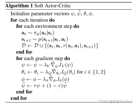
• a t ∼ π ϕ ( a t ∣ s t ) a_tsimpi_{phi}(a_t|s_t) at​∼πϕ​(at​∣st​)
  通过策略 π ϕ pi_{phi} πϕ​在依概率随机选择一个动作 a t a_t at​；
• s t + 1 ∼ p ( s t + 1 ∣ s t , a t ) s_{t+1}sim p(s_{t+1}|s_t,a_t) st+1​∼p(st+1​∣st​,at​)
  选择动作后的状态转移；
• D ∼ D ∪ { s t , a t , r ( s t , a t ) , s t + 1 } mathcal{D}simmathcal{D}cup{s_t,a_t,r(s_t,a_t),s_{t+1}} D∼D∪{st​,at​,r(st​,at​),st+1​}
  存储轨迹到经验池；
• ψ ← ψ − λ V ∇ ^ ψ J V ( ψ ) psileftarrowpsi-lambda_{V}hat{nabla}_{psi}J_{V}(psi) ψ←ψ−λV​∇^ψ​JV​(ψ)
  更新V函数网络的参数；
• θ i ← θ i − λ Q ∇ ^ θ i J Q ( θ ) , f o r   i ∈ { 1 , 2 } theta_ileftarrowtheta_i-lambda_{Q}hat{nabla}_{theta_i}J_{Q}(theta),quad for iin{1,2} θi​←θi​−λQ​∇^θi​​JQ​(θ),for i∈{1,2}
  更新Q函数网络的参数，$i=1$和$2$分别是主Q网络和目标Q网络的参数；
• ϕ ← ϕ − λ π ∇ ^ ϕ J π ( ϕ ) phileftarrowphi-lambda_{pi}hat{nabla}_{phi}J_{pi}(phi) ϕ←ϕ−λπ​∇^ϕ​Jπ​(ϕ)
  更新策略网络的参数；
• ψ ‾ ← τ ψ + ( 1 − τ ) ψ ‾ overline{psi}leftarrowtaupsi+(1-tau)overline{psi} ψ​←τψ+(1−τ)ψ​
  更新下一时间步时的V函数网络的参数，该V用于更新目标Q网络（论文公式(8)）。