离散值处理
import pandas as pd
import numpy as np
vg_df = pd.read_csv('datasets/vgsales.csv', encoding = "ISO-8859-1")
vg_df[['Name', 'Platform', 'Year', 'Genre', 'Publisher']].iloc[1:7]
|
Name |
Platform |
Year |
Genre |
Publisher |
| 1 |
Super Mario Bros. |
NES |
1985.0 |
Platform |
Nintendo |
| 2 |
Mario Kart Wii |
Wii |
2008.0 |
Racing |
Nintendo |
| 3 |
Wii Sports Resort |
Wii |
2009.0 |
Sports |
Nintendo |
| 4 |
Pokemon Red/Pokemon Blue |
GB |
1996.0 |
Role-Playing |
Nintendo |
| 5 |
Tetris |
GB |
1989.0 |
Puzzle |
Nintendo |
| 6 |
New Super Mario Bros. |
DS |
2006.0 |
Platform |
Nintendo |
genres = np.unique(vg_df['Genre'])
genres
array(['Action', 'Adventure', 'Fighting', 'Misc', 'Platform', 'Puzzle',
       'Racing', 'Role-Playing', 'Shooter', 'Simulation', 'Sports',
       'Strategy'], dtype=object)
LabelEncoder
from sklearn.preprocessing import LabelEncoder

gle = LabelEncoder()
genre_labels = gle.fit_transform(vg_df['Genre'])
genre_mappings = {index: label for index, label in enumerate(gle.classes_)}
genre_mappings
{0: 'Action',
 1: 'Adventure',
 2: 'Fighting',
 3: 'Misc',
 4: 'Platform',
 5: 'Puzzle',
 6: 'Racing',
 7: 'Role-Playing',
 8: 'Shooter',
 9: 'Simulation',
 10: 'Sports',
 11: 'Strategy'}
vg_df['GenreLabel'] = genre_labels
vg_df[['Name', 'Platform', 'Year', 'Genre', 'GenreLabel']].iloc[1:7]
|
Name |
Platform |
Year |
Genre |
GenreLabel |
| 1 |
Super Mario Bros. |
NES |
1985.0 |
Platform |
4 |
| 2 |
Mario Kart Wii |
Wii |
2008.0 |
Racing |
6 |
| 3 |
Wii Sports Resort |
Wii |
2009.0 |
Sports |
10 |
| 4 |
Pokemon Red/Pokemon Blue |
GB |
1996.0 |
Role-Playing |
7 |
| 5 |
Tetris |
GB |
1989.0 |
Puzzle |
5 |
| 6 |
New Super Mario Bros. |
DS |
2006.0 |
Platform |
4 |
Map
poke_df = pd.read_csv('datasets/Pokemon.csv', encoding='utf-8')
poke_df = poke_df.sample(random_state=1, frac=1).reset_index(drop=True)

np.unique(poke_df['Generation'])
array(['Gen 1', 'Gen 2', 'Gen 3', 'Gen 4', 'Gen 5', 'Gen 6'], dtype=object)
gen_ord_map = {'Gen 1': 1, 'Gen 2': 2, 'Gen 3': 3,
               'Gen 4': 4, 'Gen 5': 5, 'Gen 6': 6}

poke_df['GenerationLabel'] = poke_df['Generation'].map(gen_ord_map)
poke_df[['Name', 'Generation', 'GenerationLabel']].iloc[4:10]
|
Name |
Generation |
GenerationLabel |
| 4 |
Octillery |
Gen 2 |
2 |
| 5 |
Helioptile |
Gen 6 |
6 |
| 6 |
Dialga |
Gen 4 |
4 |
| 7 |
DeoxysDefense Forme |
Gen 3 |
3 |
| 8 |
Rapidash |
Gen 1 |
1 |
| 9 |
Swanna |
Gen 5 |
5 |
One-hot Encoding
poke_df[['Name', 'Generation', 'Legendary']].iloc[4:10]
|
Name |
Generation |
Legendary |
| 4 |
Octillery |
Gen 2 |
False |
| 5 |
Helioptile |
Gen 6 |
False |
| 6 |
Dialga |
Gen 4 |
True |
| 7 |
DeoxysDefense Forme |
Gen 3 |
True |
| 8 |
Rapidash |
Gen 1 |
False |
| 9 |
Swanna |
Gen 5 |
False |
from sklearn.preprocessing import OneHotEncoder, LabelEncoder
gen_le = LabelEncoder()
gen_labels = gen_le.fit_transform(poke_df['Generation'])
poke_df['Gen_Label'] = gen_labels
leg_le = LabelEncoder()
leg_labels = leg_le.fit_transform(poke_df['Legendary'])
poke_df['Lgnd_Label'] = leg_labels
poke_df_sub = poke_df[['Name', 'Generation', 'Gen_Label', 'Legendary', 'Lgnd_Label']]
poke_df_sub.iloc[4:10]
|
Name |
Generation |
Gen_Label |
Legendary |
Lgnd_Label |
| 4 |
Octillery |
Gen 2 |
1 |
False |
0 |
| 5 |
Helioptile |
Gen 6 |
5 |
False |
0 |
| 6 |
Dialga |
Gen 4 |
3 |
True |
1 |
| 7 |
DeoxysDefense Forme |
Gen 3 |
2 |
True |
1 |
| 8 |
Rapidash |
Gen 1 |
0 |
False |
0 |
| 9 |
Swanna |
Gen 5 |
4 |
False |
0 |
gen_ohe = OneHotEncoder()
gen_feature_arr = gen_ohe.fit_transform(poke_df[['Gen_Label']]).toarray()
gen_feature_labels = list(gen_le.classes_)
print (gen_feature_labels)
gen_features = pd.DataFrame(gen_feature_arr, columns=gen_feature_labels)
leg_ohe = OneHotEncoder()
leg_feature_arr = leg_ohe.fit_transform(poke_df[['Lgnd_Label']]).toarray()
leg_feature_labels = ['Legendary_'+str(cls_label) for cls_label in leg_le.classes_]
print (leg_feature_labels)
leg_features = pd.DataFrame(leg_feature_arr, columns=leg_feature_labels)
['Gen 1', 'Gen 2', 'Gen 3', 'Gen 4', 'Gen 5', 'Gen 6']
['Legendary_False', 'Legendary_True']
poke_df_ohe = pd.concat([poke_df_sub, gen_features, leg_features], axis=1)
columns = sum([['Name', 'Generation', 'Gen_Label'],gen_feature_labels,
              ['Legendary', 'Lgnd_Label'],leg_feature_labels], [])
poke_df_ohe[columns].iloc[4:10]
|
Name |
Generation |
Gen_Label |
Gen 1 |
Gen 2 |
Gen 3 |
Gen 4 |
Gen 5 |
Gen 6 |
Legendary |
Lgnd_Label |
Legendary_False |
Legendary_True |
| 4 |
Octillery |
Gen 2 |
1 |
0.0 |
1.0 |
0.0 |
0.0 |
0.0 |
0.0 |
False |
0 |
1.0 |
0.0 |
| 5 |
Helioptile |
Gen 6 |
5 |
0.0 |
0.0 |
0.0 |
0.0 |
0.0 |
1.0 |
False |
0 |
1.0 |
0.0 |
| 6 |
Dialga |
Gen 4 |
3 |
0.0 |
0.0 |
0.0 |
1.0 |
0.0 |
0.0 |
True |
1 |
0.0 |
1.0 |
| 7 |
DeoxysDefense Forme |
Gen 3 |
2 |
0.0 |
0.0 |
1.0 |
0.0 |
0.0 |
0.0 |
True |
1 |
0.0 |
1.0 |
| 8 |
Rapidash |
Gen 1 |
0 |
1.0 |
0.0 |
0.0 |
0.0 |
0.0 |
0.0 |
False |
0 |
1.0 |
0.0 |
| 9 |
Swanna |
Gen 5 |
4 |
0.0 |
0.0 |
0.0 |
0.0 |
1.0 |
0.0 |
False |
0 |
1.0 |
0.0 |
Get Dummy
gen_dummy_features = pd.get_dummies(poke_df['Generation'], drop_first=True)
pd.concat([poke_df[['Name', 'Generation']], gen_dummy_features], axis=1).iloc[4:10]
|
Name |
Generation |
Gen 2 |
Gen 3 |
Gen 4 |
Gen 5 |
Gen 6 |
| 4 |
Octillery |
Gen 2 |
1 |
0 |
0 |
0 |
0 |
| 5 |
Helioptile |
Gen 6 |
0 |
0 |
0 |
0 |
1 |
| 6 |
Dialga |
Gen 4 |
0 |
0 |
1 |
0 |
0 |
| 7 |
DeoxysDefense Forme |
Gen 3 |
0 |
1 |
0 |
0 |
0 |
| 8 |
Rapidash |
Gen 1 |
0 |
0 |
0 |
0 |
0 |
| 9 |
Swanna |
Gen 5 |
0 |
0 |
0 |
1 |
0 |
gen_onehot_features = pd.get_dummies(poke_df['Generation'])
pd.concat([poke_df[['Name', 'Generation']], gen_onehot_features], axis=1).iloc[4:10]
|
Name |
Generation |
Gen 1 |
Gen 2 |
Gen 3 |
Gen 4 |
Gen 5 |
Gen 6 |
| 4 |
Octillery |
Gen 2 |
0 |
1 |
0 |
0 |
0 |
0 |
| 5 |
Helioptile |
Gen 6 |
0 |
0 |
0 |
0 |
0 |
1 |
| 6 |
Dialga |
Gen 4 |
0 |
0 |
0 |
1 |
0 |
0 |
| 7 |
DeoxysDefense Forme |
Gen 3 |
0 |
0 |
1 |
0 |
0 |
0 |
| 8 |
Rapidash |
Gen 1 |
1 |
0 |
0 |
0 |
0 |
0 |
| 9 |
Swanna |
Gen 5 |
0 |
0 |
0 |
0 |
1 |
0 |
import pandas as pd
import matplotlib.pyplot as plt
import matplotlib as mpl
import numpy as np
import scipy.stats as spstats

%matplotlib inline
mpl.style.reload_library()
mpl.style.use('classic')
mpl.rcParams['figure.facecolor'] = (1, 1, 1, 0)
mpl.rcParams['figure.figsize'] = [6.0, 4.0]
mpl.rcParams['figure.dpi'] = 100
poke_df = pd.read_csv('datasets/Pokemon.csv', encoding='utf-8')
poke_df.head()
|
# |
Name |
Type 1 |
Type 2 |
Total |
HP |
Attack |
Defense |
Sp. Atk |
Sp. Def |
Speed |
Generation |
Legendary |
| 0 |
1 |
Bulbasaur |
Grass |
Poison |
318 |
45 |
49 |
49 |
65 |
65 |
45 |
Gen 1 |
False |
| 1 |
2 |
Ivysaur |
Grass |
Poison |
405 |
60 |
62 |
63 |
80 |
80 |
60 |
Gen 1 |
False |
| 2 |
3 |
Venusaur |
Grass |
Poison |
525 |
80 |
82 |
83 |
100 |
100 |
80 |
Gen 1 |
False |
| 3 |
3 |
VenusaurMega Venusaur |
Grass |
Poison |
625 |
80 |
100 |
123 |
122 |
120 |
80 |
Gen 1 |
False |
| 4 |
4 |
Charmander |
Fire |
NaN |
309 |
39 |
52 |
43 |
60 |
50 |
65 |
Gen 1 |
False |
poke_df[['HP', 'Attack', 'Defense']].head()
|
HP |
Attack |
Defense |
| 0 |
45 |
49 |
49 |
| 1 |
60 |
62 |
63 |
| 2 |
80 |
82 |
83 |
| 3 |
80 |
100 |
123 |
| 4 |
39 |
52 |
43 |
poke_df[['HP', 'Attack', 'Defense']].describe()
|
HP |
Attack |
Defense |
| count |
800.000000 |
800.000000 |
800.000000 |
| mean |
69.258750 |
79.001250 |
73.842500 |
| std |
25.534669 |
32.457366 |
31.183501 |
| min |
1.000000 |
5.000000 |
5.000000 |
| 25% |
50.000000 |
55.000000 |
50.000000 |
| 50% |
65.000000 |
75.000000 |
70.000000 |
| 75% |
80.000000 |
100.000000 |
90.000000 |
| max |
255.000000 |
190.000000 |
230.000000 |
popsong_df = pd.read_csv('datasets/song_views.csv', encoding='utf-8')
popsong_df.head(10)
|
user_id |
song_id |
title |
listen_count |
| 0 |
b6b799f34a204bd928ea014c243ddad6d0be4f8f |
SOBONKR12A58A7A7E0 |
You're The One |
2 |
| 1 |
b41ead730ac14f6b6717b9cf8859d5579f3f8d4d |
SOBONKR12A58A7A7E0 |
You're The One |
0 |
| 2 |
4c84359a164b161496d05282707cecbd50adbfc4 |
SOBONKR12A58A7A7E0 |
You're The One |
0 |
| 3 |
779b5908593756abb6ff7586177c966022668b06 |
SOBONKR12A58A7A7E0 |
You're The One |
0 |
| 4 |
dd88ea94f605a63d9fc37a214127e3f00e85e42d |
SOBONKR12A58A7A7E0 |
You're The One |
0 |
| 5 |
68f0359a2f1cedb0d15c98d88017281db79f9bc6 |
SOBONKR12A58A7A7E0 |
You're The One |
0 |
| 6 |
116a4c95d63623a967edf2f3456c90ebbf964e6f |
SOBONKR12A58A7A7E0 |
You're The One |
17 |
| 7 |
45544491ccfcdc0b0803c34f201a6287ed4e30f8 |
SOBONKR12A58A7A7E0 |
You're The One |
0 |
| 8 |
e701a24d9b6c59f5ac37ab28462ca82470e27cfb |
SOBONKR12A58A7A7E0 |
You're The One |
68 |
| 9 |
edc8b7b1fd592a3b69c3d823a742e1a064abec95 |
SOBONKR12A58A7A7E0 |
You're The One |
0 |
二值特征
watched = np.array(popsong_df['listen_count'])
watched[watched >= 1] = 1
popsong_df['watched'] = watched
popsong_df.head(10)
|
user_id |
song_id |
title |
listen_count |
watched |
| 0 |
b6b799f34a204bd928ea014c243ddad6d0be4f8f |
SOBONKR12A58A7A7E0 |
You're The One |
2 |
1 |
| 1 |
b41ead730ac14f6b6717b9cf8859d5579f3f8d4d |
SOBONKR12A58A7A7E0 |
You're The One |
0 |
0 |
| 2 |
4c84359a164b161496d05282707cecbd50adbfc4 |
SOBONKR12A58A7A7E0 |
You're The One |
0 |
0 |
| 3 |
779b5908593756abb6ff7586177c966022668b06 |
SOBONKR12A58A7A7E0 |
You're The One |
0 |
0 |
| 4 |
dd88ea94f605a63d9fc37a214127e3f00e85e42d |
SOBONKR12A58A7A7E0 |
You're The One |
0 |
0 |
| 5 |
68f0359a2f1cedb0d15c98d88017281db79f9bc6 |
SOBONKR12A58A7A7E0 |
You're The One |
0 |
0 |
| 6 |
116a4c95d63623a967edf2f3456c90ebbf964e6f |
SOBONKR12A58A7A7E0 |
You're The One |
17 |
1 |
| 7 |
45544491ccfcdc0b0803c34f201a6287ed4e30f8 |
SOBONKR12A58A7A7E0 |
You're The One |
0 |
0 |
| 8 |
e701a24d9b6c59f5ac37ab28462ca82470e27cfb |
SOBONKR12A58A7A7E0 |
You're The One |
68 |
1 |
| 9 |
edc8b7b1fd592a3b69c3d823a742e1a064abec95 |
SOBONKR12A58A7A7E0 |
You're The One |
0 |
0 |
from sklearn.preprocessing import Binarizer

bn = Binarizer(threshold=0.9)
pd_watched = bn.transform([popsong_df['listen_count']])[0]
popsong_df['pd_watched'] = pd_watched
popsong_df.head(11)
|
user_id |
song_id |
title |
listen_count |
watched |
pd_watched |
| 0 |
b6b799f34a204bd928ea014c243ddad6d0be4f8f |
SOBONKR12A58A7A7E0 |
You're The One |
2 |
1 |
1 |
| 1 |
b41ead730ac14f6b6717b9cf8859d5579f3f8d4d |
SOBONKR12A58A7A7E0 |
You're The One |
0 |
0 |
0 |
| 2 |
4c84359a164b161496d05282707cecbd50adbfc4 |
SOBONKR12A58A7A7E0 |
You're The One |
0 |
0 |
0 |
| 3 |
779b5908593756abb6ff7586177c966022668b06 |
SOBONKR12A58A7A7E0 |
You're The One |
0 |
0 |
0 |
| 4 |
dd88ea94f605a63d9fc37a214127e3f00e85e42d |
SOBONKR12A58A7A7E0 |
You're The One |
0 |
0 |
0 |
| 5 |
68f0359a2f1cedb0d15c98d88017281db79f9bc6 |
SOBONKR12A58A7A7E0 |
You're The One |
0 |
0 |
0 |
| 6 |
116a4c95d63623a967edf2f3456c90ebbf964e6f |
SOBONKR12A58A7A7E0 |
You're The One |
17 |
1 |
1 |
| 7 |
45544491ccfcdc0b0803c34f201a6287ed4e30f8 |
SOBONKR12A58A7A7E0 |
You're The One |
0 |
0 |
0 |
| 8 |
e701a24d9b6c59f5ac37ab28462ca82470e27cfb |
SOBONKR12A58A7A7E0 |
You're The One |
68 |
1 |
1 |
| 9 |
edc8b7b1fd592a3b69c3d823a742e1a064abec95 |
SOBONKR12A58A7A7E0 |
You're The One |
0 |
0 |
0 |
| 10 |
fb41d1c374d093ab643ef3bcd70eeb258d479076 |
SOBONKR12A58A7A7E0 |
You're The One |
1 |
1 |
1 |
多项式特征
atk_def = poke_df[['Attack', 'Defense']]
atk_def.head()
|
Attack |
Defense |
| 0 |
49 |
49 |
| 1 |
62 |
63 |
| 2 |
82 |
83 |
| 3 |
100 |
123 |
| 4 |
52 |
43 |
from sklearn.preprocessing import PolynomialFeatures

pf = PolynomialFeatures(degree=2, interaction_only=False, include_bias=False)
res = pf.fit_transform(atk_def)
res
array([[    49.,     49.,   2401.,   2401.,   2401.],
       [    62.,     63.,   3844.,   3906.,   3969.],
       [    82.,     83.,   6724.,   6806.,   6889.],
       ...,
       [   110.,     60.,  12100.,   6600.,   3600.],
       [   160.,     60.,  25600.,   9600.,   3600.],
       [   110.,    120.,  12100.,  13200.,  14400.]])
intr_features = pd.DataFrame(res, columns=['Attack', 'Defense', 'Attack^2', 'Attack x Defense', 'Defense^2'])
intr_features.head(5)
|
Attack |
Defense |
Attack^2 |
Attack x Defense |
Defense^2 |
| 0 |
49.0 |
49.0 |
2401.0 |
2401.0 |
2401.0 |
| 1 |
62.0 |
63.0 |
3844.0 |
3906.0 |
3969.0 |
| 2 |
82.0 |
83.0 |
6724.0 |
6806.0 |
6889.0 |
| 3 |
100.0 |
123.0 |
10000.0 |
12300.0 |
15129.0 |
| 4 |
52.0 |
43.0 |
2704.0 |
2236.0 |
1849.0 |
binning特征
fcc_survey_df = pd.read_csv('datasets/fcc_2016_coder_survey_subset.csv', encoding='utf-8')
fcc_survey_df[['ID.x', 'EmploymentField', 'Age', 'Income']].head()
|
ID.x |
EmploymentField |
Age |
Income |
| 0 |
cef35615d61b202f1dc794ef2746df14 |
office and administrative support |
28.0 |
32000.0 |
| 1 |
323e5a113644d18185c743c241407754 |
food and beverage |
22.0 |
15000.0 |
| 2 |
b29a1027e5cd062e654a63764157461d |
finance |
19.0 |
48000.0 |
| 3 |
04a11e4bcb573a1261eb0d9948d32637 |
arts, entertainment, sports, or media |
26.0 |
43000.0 |
| 4 |
9368291c93d5d5f5c8cdb1a575e18bec |
education |
20.0 |
6000.0 |
fig, ax = plt.subplots()
fcc_survey_df['Age'].hist(color='#A9C5D3')
ax.set_title('Developer Age Histogram', fontsize=12)
ax.set_xlabel('Age', fontsize=12)
ax.set_ylabel('Frequency', fontsize=12)
Text(0,0.5,'Frequency')
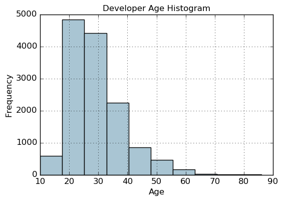
Binning based on rounding
Age Range: Bin
---------------
 0 -  9  : 0
10 - 19  : 1
20 - 29  : 2
30 - 39  : 3
40 - 49  : 4
50 - 59  : 5
60 - 69  : 6
  ... and so on
fcc_survey_df['Age_bin_round'] = np.array(np.floor(np.array(fcc_survey_df['Age']) / 10.))
fcc_survey_df[['ID.x', 'Age', 'Age_bin_round']].iloc[1071:1076]
|
ID.x |
Age |
Age_bin_round |
| 1071 |
6a02aa4618c99fdb3e24de522a099431 |
17.0 |
1.0 |
| 1072 |
f0e5e47278c5f248fe861c5f7214c07a |
38.0 |
3.0 |
| 1073 |
6e14f6d0779b7e424fa3fdd9e4bd3bf9 |
21.0 |
2.0 |
| 1074 |
c2654c07dc929cdf3dad4d1aec4ffbb3 |
53.0 |
5.0 |
| 1075 |
f07449fc9339b2e57703ec7886232523 |
35.0 |
3.0 |
分位数切分
fcc_survey_df[['ID.x', 'Age', 'Income']].iloc[4:9]
|
ID.x |
Age |
Income |
| 4 |
9368291c93d5d5f5c8cdb1a575e18bec |
20.0 |
6000.0 |
| 5 |
dd0e77eab9270e4b67c19b0d6bbf621b |
34.0 |
40000.0 |
| 6 |
7599c0aa0419b59fd11ffede98a3665d |
23.0 |
32000.0 |
| 7 |
6dff182db452487f07a47596f314bddc |
35.0 |
40000.0 |
| 8 |
9dc233f8ed1c6eb2432672ab4bb39249 |
33.0 |
80000.0 |
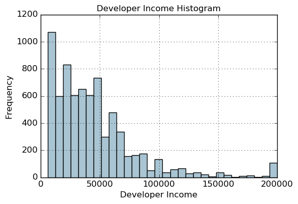
fig, ax = plt.subplots()
fcc_survey_df['Income'].hist(bins=30, color='#A9C5D3')
ax.set_title('Developer Income Histogram', fontsize=12)
ax.set_xlabel('Developer Income', fontsize=12)
ax.set_ylabel('Frequency', fontsize=12)
Text(0,0.5,'Frequency')
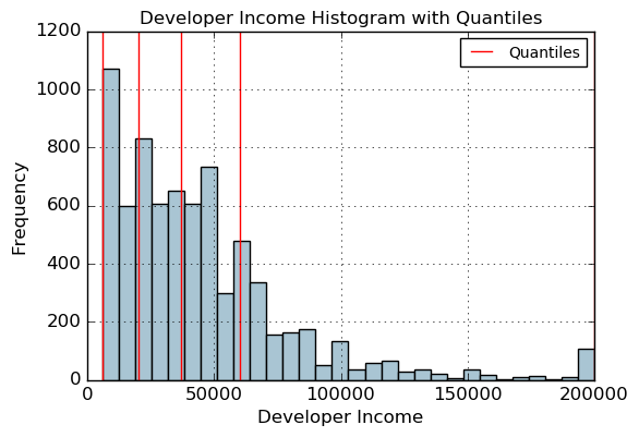
quantile_list = [0, .25, .5, .75, 1.]
quantiles = fcc_survey_df['Income'].quantile(quantile_list)
quantiles
0.00      6000.0
0.25     20000.0
0.50     37000.0
0.75     60000.0
1.00    200000.0
Name: Income, dtype: float64
fig, ax = plt.subplots()
fcc_survey_df['Income'].hist(bins=30, color='#A9C5D3')

for quantile in quantiles:
    qvl = plt.axvline(quantile, color='r')
ax.legend([qvl], ['Quantiles'], fontsize=10)

ax.set_title('Developer Income Histogram with Quantiles', fontsize=12)
ax.set_xlabel('Developer Income', fontsize=12)
ax.set_ylabel('Frequency', fontsize=12)
Text(0,0.5,'Frequency')
quantile_labels = ['0-25Q', '25-50Q', '50-75Q', '75-100Q']
fcc_survey_df['Income_quantile_range'] = pd.qcut(fcc_survey_df['Income'],
                                                 q=quantile_list)
fcc_survey_df['Income_quantile_label'] = pd.qcut(fcc_survey_df['Income'],
                                                 q=quantile_list, labels=quantile_labels)
fcc_survey_df[['ID.x', 'Age', 'Income',
               'Income_quantile_range', 'Income_quantile_label']].iloc[4:9]
|
ID.x |
Age |
Income |
Income_quantile_range |
Income_quantile_label |
| 4 |
9368291c93d5d5f5c8cdb1a575e18bec |
20.0 |
6000.0 |
(5999.999, 20000.0] |
0-25Q |
| 5 |
dd0e77eab9270e4b67c19b0d6bbf621b |
34.0 |
40000.0 |
(37000.0, 60000.0] |
50-75Q |
| 6 |
7599c0aa0419b59fd11ffede98a3665d |
23.0 |
32000.0 |
(20000.0, 37000.0] |
25-50Q |
| 7 |
6dff182db452487f07a47596f314bddc |
35.0 |
40000.0 |
(37000.0, 60000.0] |
50-75Q |
| 8 |
9dc233f8ed1c6eb2432672ab4bb39249 |
33.0 |
80000.0 |
(60000.0, 200000.0] |
75-100Q |
对数变换 COX-BOX
fcc_survey_df['Income_log'] = np.log((1+ fcc_survey_df['Income']))
fcc_survey_df[['ID.x', 'Age', 'Income', 'Income_log']].iloc[4:9]
|
ID.x |
Age |
Income |
Income_log |
| 4 |
9368291c93d5d5f5c8cdb1a575e18bec |
20.0 |
6000.0 |
8.699681 |
| 5 |
dd0e77eab9270e4b67c19b0d6bbf621b |
34.0 |
40000.0 |
10.596660 |
| 6 |
7599c0aa0419b59fd11ffede98a3665d |
23.0 |
32000.0 |
10.373522 |
| 7 |
6dff182db452487f07a47596f314bddc |
35.0 |
40000.0 |
10.596660 |
| 8 |
9dc233f8ed1c6eb2432672ab4bb39249 |
33.0 |
80000.0 |
11.289794 |
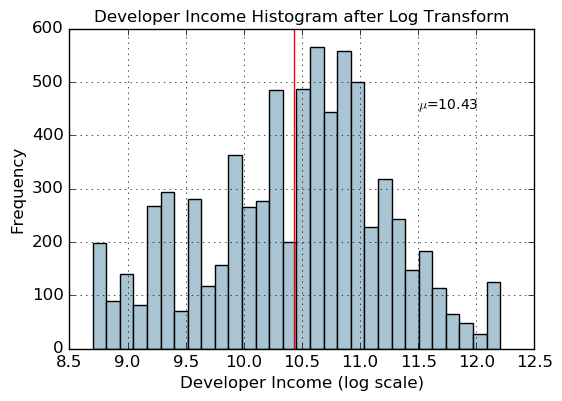
income_log_mean = np.round(np.mean(fcc_survey_df['Income_log']), 2)

fig, ax = plt.subplots()
fcc_survey_df['Income_log'].hist(bins=30, color='#A9C5D3')
plt.axvline(income_log_mean, color='r')
ax.set_title('Developer Income Histogram after Log Transform', fontsize=12)
ax.set_xlabel('Developer Income (log scale)', fontsize=12)
ax.set_ylabel('Frequency', fontsize=12)
ax.text(11.5, 450, r'$mu$='+str(income_log_mean), fontsize=10)
Text(11.5,450,'$\mu$=10.43')
日期相关特征
import datetime
import numpy as np
import pandas as pd
from dateutil.parser import parse
import pytz
time_stamps = ['2015-03-08 10:30:00.360000+00:00', '2017-07-13 15:45:05.755000-07:00',
               '2012-01-20 22:30:00.254000+05:30', '2016-12-25 00:30:00.000000+10:00']
df = pd.DataFrame(time_stamps, columns=['Time'])
df
|
Time |
| 0 |
2015-03-08 10:30:00.360000+00:00 |
| 1 |
2017-07-13 15:45:05.755000-07:00 |
| 2 |
2012-01-20 22:30:00.254000+05:30 |
| 3 |
2016-12-25 00:30:00.000000+10:00 |
ts_objs = np.array([pd.Timestamp(item) for item in np.array(df.Time)])
df['TS_obj'] = ts_objs
ts_objs
array([Timestamp('2015-03-08 10:30:00.360000+0000', tz='UTC'),
       Timestamp('2017-07-13 15:45:05.755000-0700', tz='pytz.FixedOffset(-420)'),
       Timestamp('2012-01-20 22:30:00.254000+0530', tz='pytz.FixedOffset(330)'),
       Timestamp('2016-12-25 00:30:00+1000', tz='pytz.FixedOffset(600)')], dtype=object)
df['Year'] = df['TS_obj'].apply(lambda d: d.year)
df['Month'] = df['TS_obj'].apply(lambda d: d.month)
df['Day'] = df['TS_obj'].apply(lambda d: d.day)
df['DayOfWeek'] = df['TS_obj'].apply(lambda d: d.dayofweek)
df['DayName'] = df['TS_obj'].apply(lambda d: d.weekday_name)
df['DayOfYear'] = df['TS_obj'].apply(lambda d: d.dayofyear)
df['WeekOfYear'] = df['TS_obj'].apply(lambda d: d.weekofyear)
df['Quarter'] = df['TS_obj'].apply(lambda d: d.quarter)

df[['Time', 'Year', 'Month', 'Day', 'Quarter',
    'DayOfWeek', 'DayName', 'DayOfYear', 'WeekOfYear']]
|
Time |
Year |
Month |
Day |
Quarter |
DayOfWeek |
DayName |
DayOfYear |
WeekOfYear |
| 0 |
2015-03-08 10:30:00.360000+00:00 |
2015 |
3 |
8 |
1 |
6 |
Sunday |
67 |
10 |
| 1 |
2017-07-13 15:45:05.755000-07:00 |
2017 |
7 |
13 |
3 |
3 |
Thursday |
194 |
28 |
| 2 |
2012-01-20 22:30:00.254000+05:30 |
2012 |
1 |
20 |
1 |
4 |
Friday |
20 |
3 |
| 3 |
2016-12-25 00:30:00.000000+10:00 |
2016 |
12 |
25 |
4 |
6 |
Saturday |
360 |
51 |
时间相关特征
df['Hour'] = df['TS_obj'].apply(lambda d: d.hour)
df['Minute'] = df['TS_obj'].apply(lambda d: d.minute)
df['Second'] = df['TS_obj'].apply(lambda d: d.second)
df['MUsecond'] = df['TS_obj'].apply(lambda d: d.microsecond)
df['UTC_offset'] = df['TS_obj'].apply(lambda d: d.utcoffset())
df[['Time', 'Hour', 'Minute', 'Second', 'MUsecond', 'UTC_offset']]
|
Time |
Hour |
Minute |
Second |
MUsecond |
UTC_offset |
| 0 |
2015-03-08 10:30:00.360000+00:00 |
10 |
30 |
0 |
360000 |
00:00:00 |
| 1 |
2017-07-13 15:45:05.755000-07:00 |
15 |
45 |
5 |
755000 |
-1 days +17:00:00 |
| 2 |
2012-01-20 22:30:00.254000+05:30 |
22 |
30 |
0 |
254000 |
05:30:00 |
| 3 |
2016-12-25 00:30:00.000000+10:00 |
0 |
30 |
0 |
0 |
10:00:00 |
按照早晚切分时间
hour_bins = [-1, 5, 11, 16, 21, 23]
bin_names = ['Late Night', 'Morning', 'Afternoon', 'Evening', 'Night']
df['TimeOfDayBin'] = pd.cut(df['Hour'],
                            bins=hour_bins, labels=bin_names)
df[['Time', 'Hour', 'TimeOfDayBin']]
|
Time |
Hour |
TimeOfDayBin |
| 0 |
2015-03-08 10:30:00.360000+00:00 |
10 |
Morning |
| 1 |
2017-07-13 15:45:05.755000-07:00 |
15 |
Afternoon |
| 2 |
2012-01-20 22:30:00.254000+05:30 |
22 |
Night |
| 3 |
2016-12-25 00:30:00.000000+10:00 |
0 |
Late Night |